Authors: Kenneth Marino, Ruslan Salakhutdinov, Abhinav Gupta
Paper reference: https://arxiv.org/pdf/1612.04844.pdf
Overview
Note: This previous post I wrote might be helpful for reading this paper summary:
This paper investigates the use of structured prior knowledge in the form of knowledge graphs and shows that using this knowledge improves performance on image classification.
It introduce the Graph Search Neural Network (GSNN) as a way of efficiently incorporating large knowledge graphs into a vision classification pipeline, which outperforms standard neural network baselines for multi-label classification.
Intuition
While modern learning-based approaches can recognize some categories with high accuracy, it usually requires thousands of labeled examples for each of these categories. This approach of building large datasets for every concept is unscalable. One way to solve this problem is to use structured knowledge and reasoning (prior knowledge, this is what human usually do but current approaches do not).
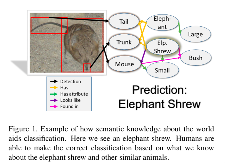
For example, when people try to identify the animal shown in the figure, they will first recognize the animal, then recall relevant knowledge, and finally reason about it. With this information, even if we have only seen one or two pictures of this animal, we would be able to classify it. So we hope a model could also have similar reasoning process.
Previous Work
There has been a lot of work in end-to-end learning on graphs or neural network trained on graphs. Most of these approaches either extract features from the graph or they learn a propagation model that transfers evidence between nodes conditional on the type of edge. An example of this is the Gated Graph Neural Network which takes an arbitrary graph as input. Given some initialization specific to the task, it learns how to propagate information and predict the output for every node in the graph.
Previous works are focusing on building and then querying knowledge bases rather than using existing knowledge bases as side information for some vision task.
This work not only uses attribute relationships that appear in our knowledge graphs, but also uses relationships between objects and reasons directly on graphs rather than using object-attribute pairs directly.
Major Contribution
-
The introduction of the GSNN as a way of incorporating potentially large knowledge graphs into an end-to-end learning system that is computationally feasible for large graphs;
-
Provide a framework for using noisy knowledge graphs for image classification (In vision problems, graphs encode contextual and common-sense relationships and are significantly larger and noisier);
-
The ability to explain image classifications by using the propagation model (Interpretability).
Graph Search Neural Network (GSNN)
GSNN Explanation
The idea is that rather than performing the recurrent update over all of the nodes of the graph at once, it starts with some initial nodes based on the input and only choose to expand nodes which are useful for the final output. Thus, the model only compute the update steps over a subset of the graph.
Steps in GSNN:
- Determine Initial Nodes
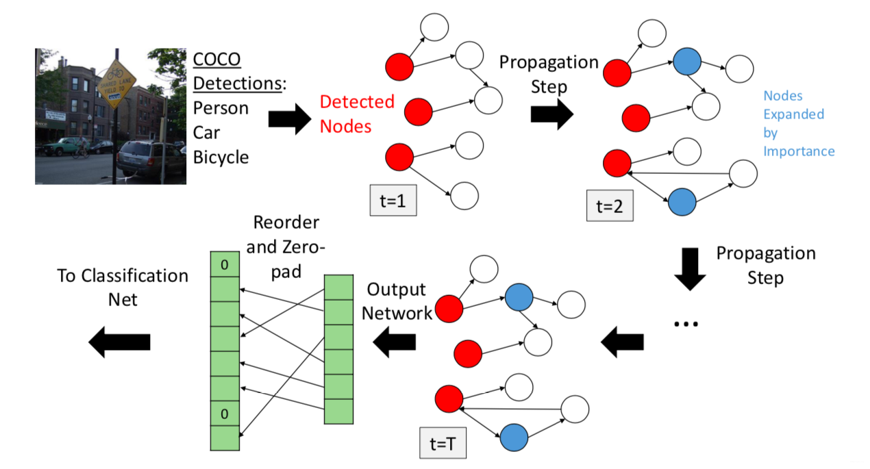
They determine initial nodes in the graph based on likelihood of the visual concept being present as determined by an object detector or classifier. For their experiments, they use Faster R-CNN for each of the 80 COCO categories. For scores over some chosen threshold, they choose the corresponding nodes in the graph as our initial set of active nodes. Once they have initial nodes, they also add the nodes adjacent to the initial nodes to the active set.
- Propagation
Given the initial nodes, they want to first propagate the beliefs about the initial nodes to all of the adjacent nodes (propagation network). This process is similar to GGNN.
- Decide which nodes to expand next
After the first time step, they need a way of deciding which nodes to expand next. Therefore, a per-node scoring function is learned to estimates how “important” that node is. After each propagation step, for every node in the current graph, the model predict an importance score
$$ i_{v}^{(t)}=g_{i}\left(h_{v}, x_{v}\right) $$
where $g_{i}$ is a learned network, the importance network. Once we have values of $i_{v}$, we take the top $P$ scoring nodes that have never been expanded and add them to the expanded set, and add all nodes adjacent to those nodes to our active set.
The above two steps (Propagation, Decide which nodes to expand next) repeated $T$ times ($T$ is a hyper-parameter).
Lastly, at the final time step $T$, the model computes the per-node-output (output network) and re-order and zero-pad the outputs into the final classification net. Re-order it so that nodes always appear in the same order into the final network, and zero pad any nodes that were not expanded.
The entire process is shown in the figure above.
Three networks
-
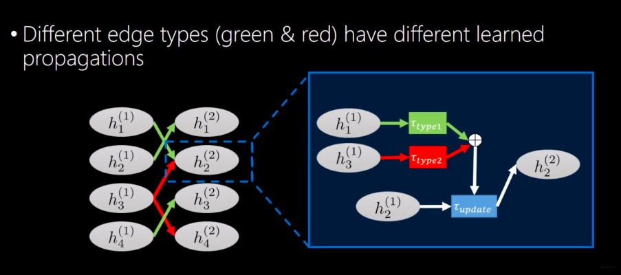
Propagation network: normal Graph Gated Neural Network (GGNN). GGNN is a fully end-to-end network that takes as input a directed graph and outputs either a classification over the entire graph or an output for each node. Check my previous post to know more details about GGNN and how propagation works.
-
Output network: After $T$ time steps, we have our final hidden states. The node level outputs can then just be computed as $$ o_{v}=g\left(h_{v}^{(T)}, x_{v}\right) $$ where $g$ is a fully connected network, the output network, and $x_{v}$ is the original annotation for the node.
-
Importance network: learn a per-node scoring function that estimates how “important” that node is. To train the importance net, they assign target importance value to each node in the graph for a given image. Nodes corresponding to ground-truth concepts in an image are assigned an importance value of 1. The neighbors of these nodes are assigned a value of $\gamma$. Nodes which are two-hop away have value $\gamma^2$ and so on. The idea is that nodes closest to the final output are the most important to expand. After each propagation step, for each node in the current graph, they predict an importance score $$ i_{v}^{(t)}=g_{i}\left(h_{v}, x_{v}\right) $$
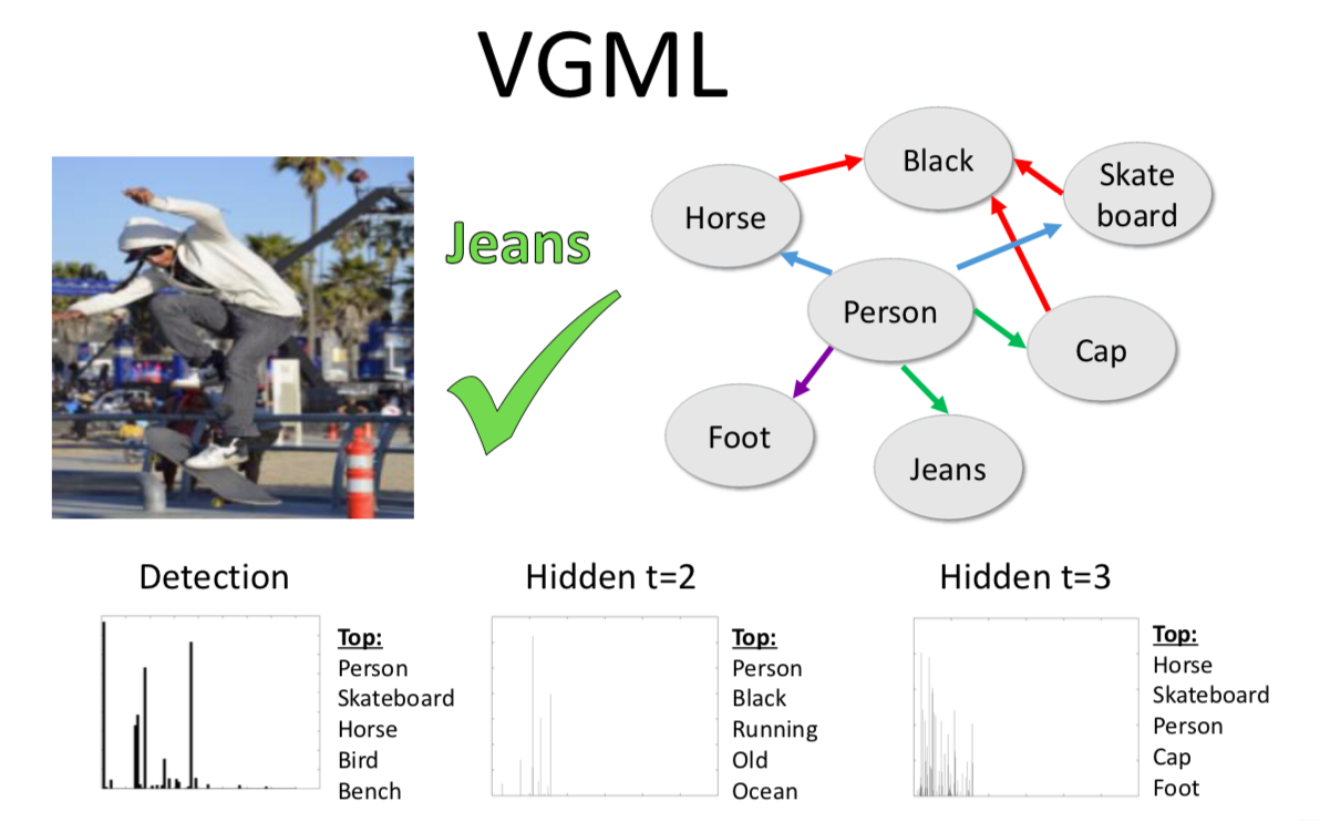
Diagram visualization
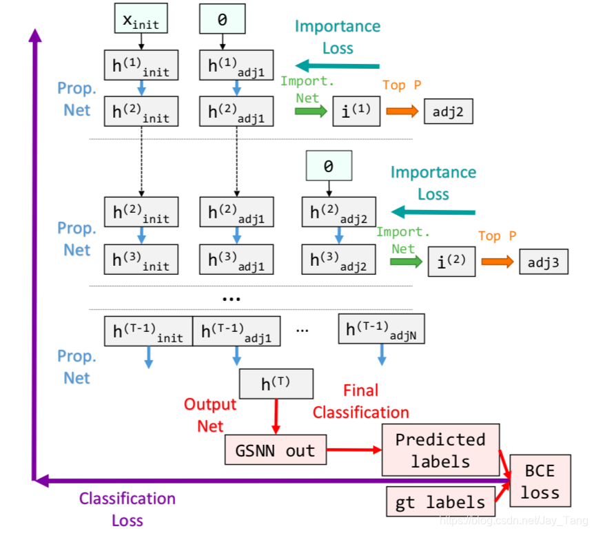
First $x_{init}$, the detection confidences initialize $h_{i n i t}^{(1)}$, the hidden states of the initially detected nodes (Each visual concept (e.x., person, horse, cat, etc) in the knowledge graph is represented in a hidden state). We then initialize $h_{a d j 1}^{(1)}$, the hidden states of the adjacent nodes, with $0$. We then update the hidden states using the propagation net. The values of $h^{(2)}$ are then used to predict the importance scores $i^{(1)}$ which are used to pick the next nodes to add $adj2$. These nodes are then initialized with $h_{a d j 2}^{(2)}=0$ and the hidden states are updated again through the propagation net. After $T$ steps, we then take all of the accumulated hidden states $h^{T}$ to predict the GSNN outputs for all the active nodes. During backpropagation, the binary cross entropy (BCE) loss is fed backward through the output layer, and the importance losses are fed through the importance networks to update the network parameters.
One final detail is the addition of a “node bias” into GSNN. In GGNN, the per-node output function $g\left(h_{v}^{(T)}, x_{v}\right)$, takes in the hidden state and initial annotation of the node $v$ to compute its output. Our output equations are now $g\left(h_{v}^{(T)}, x_{v}, n_{v}\right)$ where $n_{v}$ is a bias term that is tied to a particular node $v$ in the overall graph. This value is stored in a table and its value are updated by backpropagation.
Advantage
-
This new architecture mitigates the computational issues with the Gated Graph Neural Networks for large graphs which allows our model to be efficiently trained for image tasks using large knowledge graphs.
-
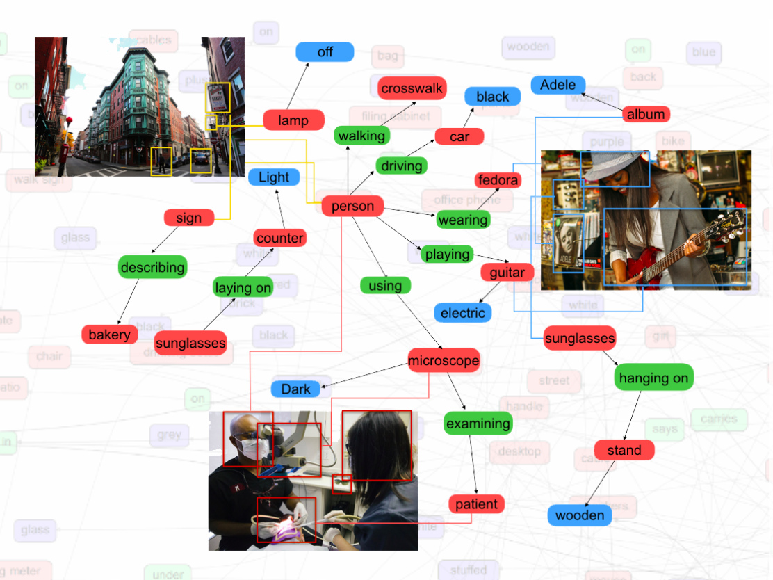
Importantly, the GSNN model is also able to provide explanations on classifications by following how the information is propagated in the graph.
Incorporate the graph network into an image pipeline
We take the output of the graph network, re-order it so that nodes always appear in the same order into the final network, and zero pad any nodes that were not expanded. Therefore, if we have a graph with 316 node outputs, and each node predicts a 5-dim hidden variable, we create a 1580-dim feature vector from the graph. We also concatenate this feature vector with fc7 layer (4096-dim) of a fine-tuned VGG-16 network and top-score for each COCO category predicted by Faster R-CNN (80-dim). This 5756-dim feature vector is then fed into 1-layer final classification network trained with dropout.
You can think of this as a way of feature engineering where you concatenate the output from models with different structures.
Dataset
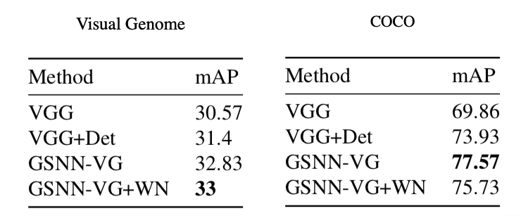
COCO: COCO is a large-scale object detection, segmentation, and captioning dataset, which includes 80 object categories.
Visual Genome: a dataset that represents the complex, noisy visual world with its many different kinds of objects, where labels are potentially ambiguous and overlapping, and categories fall into a long-tail distribution (skew to the right).
Visual Genome contains over 100,000 natural images from the Internet. Each image is labeled with objects, attributes and relationships between objects entered by human annotators. They create a subset from Visual Genome which they call Visual Genome multi-label dataset or VGML (They took 316 visual concepts from the subset).
Using only the train split, we build a knowledge graph connecting the concepts using the most common object-attribute and object-object relationships in the dataset. Specifically, we counted how often an object/object relationship or object/attribute pair occurred in the training set, and pruned any edges that had fewer than 200 instances. This leaves us with a graph over all of the images with each edge being a common relationship.
Visual Genome + WordNet: including the outside semantic knowledge from WordNet. The Visual Genome graphs do not contain useful semantic relationships. For instance, it might be helpful to know that dog is an animal if our visual system sees a dog and one of our labels is animal. Check the original paper to know how to add WordNet into the graph.
Conclusion
In this paper, they present the Graph Search Neural Network (GSNN) as a way of efficiently using knowledge graphs as extra information to improve image classification.
Next Step:
The GSNN and the framework they use for vision problems is completely general. The next steps will be to apply the GSNN to other vision tasks, such as detection, Visual Question Answering, and image captioning.
Another interesting direction would be to combine the procedure of this work with a system such as NEIL to create a system which builds knowledge graphs and then prunes them to get a more accurate, useful graph for image tasks.
Reference:
- Visual Genome: https://visualgenome.org
- The More You Know: Using Knowledge Graphs for Image Classification: https://arxiv.org/abs/1612.04844