Linear SVM

Idea
We want to find a hyper-plane $w^\top x + b = 0$ that maximizes the margin.
Set up
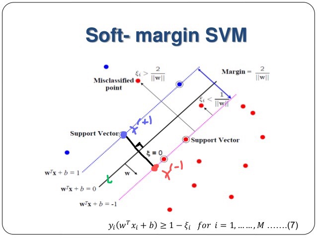
We first show that the vector $w$ is orthogonal to this hyper-plane. Let $x_1$, $x_2$ be any element on the hyper-plane. So we have $w^\top x_1 + b = 0$ and $w^\top x_2 + b = 0$. Then $w^\top (x_1 - x_2) = 0$, which implies $w$ is orthogonal to the hyper-plane. Now, we set two dashed lines to $w^\top x + b = 1$ and $w^\top x + b = -1$. In fact, “$1$” doesn’t matter and we can pick any value here. “$1$” is just the convention.
Now we pick any line parallel (orthogonal) to $w$ (hyper-plane), then the line intersect two dashed line with point $x^{(+)}$ and $x^{(-)}$. We want to maximize the margin
$$margin = || x^{(+)} - x^{(-)}||$$
Re-express margin
Since $w$ is parallel to $x^{(+)} - x^{(-)}$, we have $x^{(+)} - x^{(-)}$ = $\lambda w$ for some $\lambda$. Then
$$x^{(+)} = \lambda w + x^{(-)}$$
Since $w^\top x^{(+)} + b = 1$, we have $w^\top (\lambda w + x^{(-)}) + b = 1$ and then $\lambda w^\top w + w^\top x^{(-)} + b = 1$. Since $w^\top x^{(-)} + b = -1$, we have $\lambda = w^\top w = 2$. So
$$ \lambda = \frac{2}{w^\top w}$$
Now we can rewrite the margin as
$$ margin = ||(\lambda w + x^{(-)}) - x^{(-)}|| = ||\lambda w|| = ||\frac{2}{w^\top w} w || = \frac{2}{||w||}$$
Construct an optimization problem
we can construct the following objective function for SVM:

we can re-write it as

Soft version of linear SVM
Note that the above constraints are hard constraints and it only works if the data are linearly separable.
Therefore, if data is not linearly separable, we want to make a soft constraint (relaxation). That is, we allow the model to make some error, but we will add some penalty for them.

Note that if $\lambda \to \infty$, then we allow no error; if $\lambda = 0$, then we add no penalty. We call $\epsilon_i$ a slack variable. Ideally, we want $\epsilon_i = 0$; if it makes an error, $\epsilon_i > 0$.
Convert to Hinge Loss
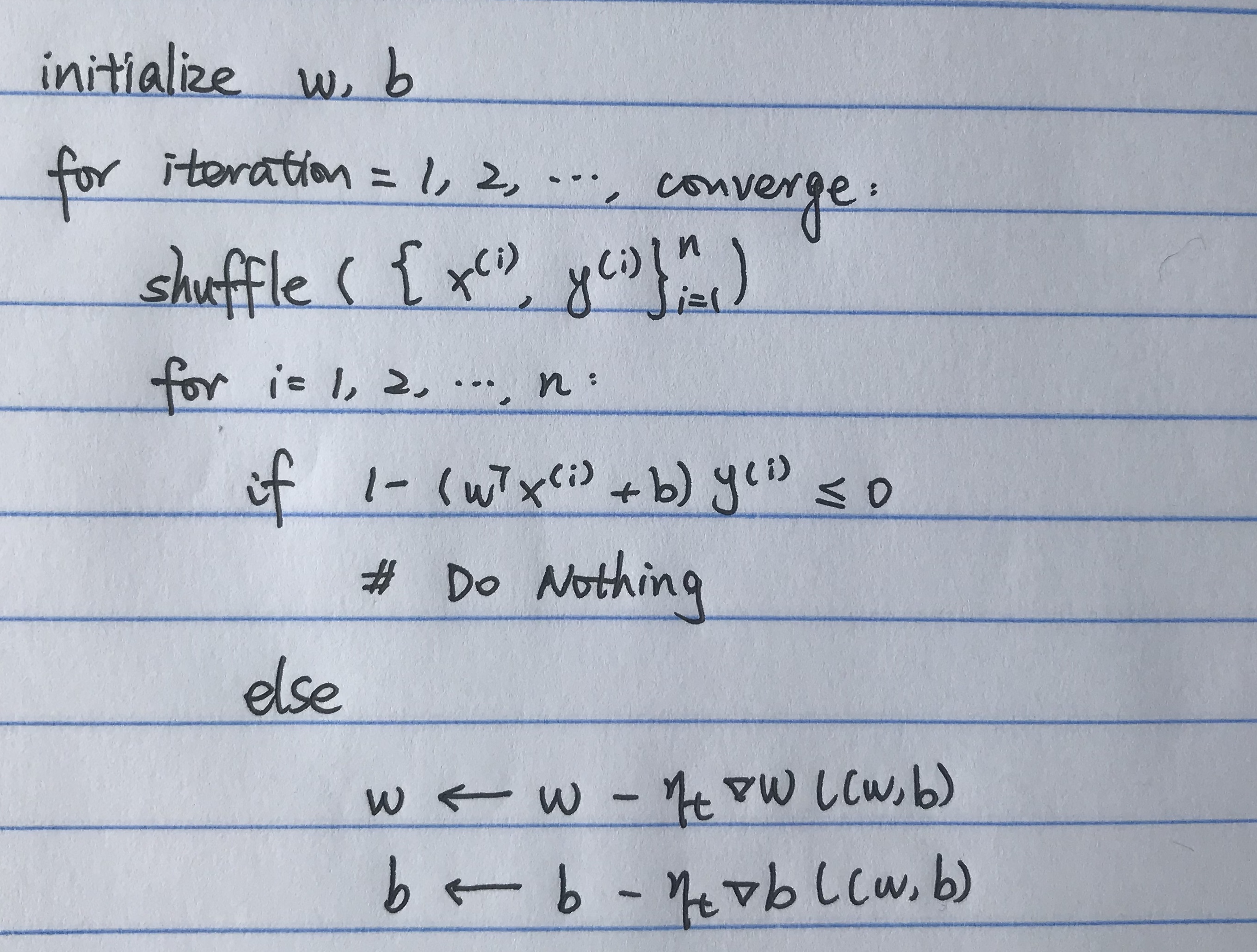
Since $(w^\top x^{(i)} + b)y^{(i)} \geq 1 - \epsilon_i$, we have $\epsilon_i \geq 1-(w^\top x^{(i)} + b)y^{(i)}$. If $\epsilon_i \leq 0$, we have no loss. Otherwise, we add $\epsilon_i = 1-(w^\top x^{(i)} + b)y^{(i)}$ as loss. So right now our new objective function is

Stochastic Gradient descent for Hinge Loss objective function:

Non-linear SVM
We are going to map all points through a non-linear function and then used SVM in this transformed space. The idea is that if the non-linear map we use maps the two sets of points such that the two sets of points can be separated by a line after the transformation, then SVM can be used in this transformed space instead of the original space.
Let $\phi: \mathcal{X} \to \mathcal{F}$ be the non linear map described in the earlier paragraph, where $\mathcal{X}$ is the space from which inputs points are coming from and $\mathcal{F}$ is the transformed space. For SVM to work, we don’t need to know $\phi$ explicitly, but only need to know the dot product of the transformed points $⟨\phi(x_i), \phi(x_j)⟩$. So, instead of working with $\phi$, they can instead work with $K: \mathcal{X} \times \mathcal{X} \to \mathbb{R}$ where $K$ takes two points as input and returns a real value that represents $⟨\phi(x_i), \phi(x_j)⟩$. Note that $\phi$ exists only when $K$ is positive definite. With this, we are able to run SVM on an infinite dimensional space.
Gram Matrix: Given a set of vectors in $\mathcal{V}$, the Gram Matrix is the matrix of all possible inner products in $\mathcal{V}$. That is, $G_{ij} = v_i \cdot v_j$.
Curse of Dimensionality
As the dimensionality increases, the classifier’s performance increases until the optimal number of features is reached. Further increasing the dimensionality without increasing the number of training samples results in a decrease in classifier performance. The common theme of these problems is that when the dimensionality increases, the volume of the space increases so fast that the available data become sparse. In order to obtain a statistically sound and reliable result, the amount of data needed to support the result often grows exponentially with the dimensionality. Also, the time complexity of a classification algorithm is proportional to the dimension of the data point. So, higher dimension means larger time complexity (not to mention space complexity to store those large dimensional points).
Mercer’s Theorem (simplified idea): In a finite input space, if the Kernel matrix $\mathbf{K}$ (also known as Gram matrix) is positive semi-definite ($\mathbf{K}_{ij} = K(x_i, x_j) = \phi(x_i) \cdot \phi(x_j)$), then the matrix element, i.e. the function K, can be a kernel function.
Example of a kernel function
Let $x_i = (x_{i1}, x_{i2}), x_j = (x_{j1}, x_{j2})$ and $\phi(x_i)=(x_{i1}^2, \sqrt{2}x_{i1}x_{i2}, x_{i2}^2), \phi(x_j)=(x_{j1}^2, \sqrt{2}x_{j1}x_{j2}, x_{j2}^2)$. Then

From this example, we see that even if the dimension of the feature space is higher than the input space, we can still do the computation in the low dimension input space as long as we choose a good kernel! Therefore, it’s possible to run SVM on an infinite dimensional feature space but do the same amount of computation as in the low dimension input space if we choose a good kernel.
Note:
- Let $n$ be the dimension of input space, $N (» n)$ be the dimension of the feature space, then if we choose a kernel $K$ properly, we are able to compute the dot product in higher dimensional space but in complexity $O(n)$ instead of $O(N)$.
- If the classification algorithm is only dependent on the dot product and has no dependency on the actual map $\phi$, I can use the kernel trick to run the algorithm in high dimensional space with almost no additional cost.
Common Kernel Function
Polynomial Kernel
$$k(x_i, x_j) = (x_i \cdot x_j + 1)^d$$
where $d$ is the degree of the polynomial. This type of kernel represents the similarity of vectors in a feature space over polynomials of the original variables. It is popular in natural language processing.
Gaussian Kernel
$$k(x, y) = \text{exp}\left(-\frac{|x_i - x_j|^2}{2\sigma^2}\right)$$
This type of kernel is useful when there is no prior knowledge about the data; it has good performance when there is the assumption og general smoothness of the data. It is an example of the radial basis function kernel (below). $\sigma$ is the regularization variable that can be tuned specifically for each problem.
Gaussian Radial Basis Function (RBF)
$$k(x_i, x_j) = \text{exp}(-\gamma |x_i - x_j|^2)$$
for $\gamma > 0$. The difference between this kernel and the gaussian kernel is the amount of regularization applied.
Exponential Kernel
$$k(x, y) = \text{exp}\left(-\frac{|x_i - x_j|}{2\sigma^2}\right)$$
Dual problem of SVM
Our primal problem is

Note that the primal problem of SVM is a convex problem and the constraints are convex. We know that for any convex optimization problem with differentiable objective and constraint functions, any points that satisfy the KKT conditions are primal and dual optimal, and have zero duality gap.
We can re-write the primal problem as

where $\phi(x_i)$ is a map of $x_i$ from input space to feature space. Now

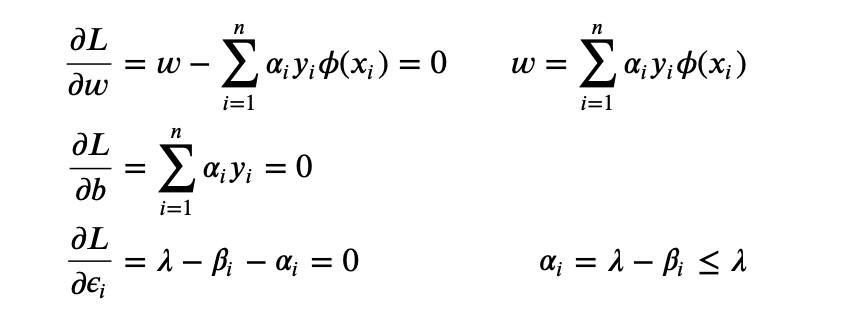
Then we can use the $4$-th KKT condition (gradient w.r.t. $w, b, \epsilon_i$ is $0$):

Therefore we have

Our dual problem of SVM is

Note that the maximization only depends on the dot product of $\phi(x_i), \phi(x_j)$. We define a function
$$K(x_i, x_j) = \phi(x_i) \cdot \phi(x_j)$$
All we need is the function $K$, a kernel function, which provides with the dot product of two vectors in another space and we don’t need to know the transformation into the other space.
We can re-write the problem as

Reference:
- https://www.quora.com/Why-should-a-kernel-function-satisfy-Mercers-condition
- https://scikit-learn.org/stable/modules/svm.html#svm-kernels
- https://kfrankc.com/posts/2019/06/21/kernel-functions-svm#
- https://towardsdatascience.com/understanding-support-vector-machine-part-2-kernel-trick-mercers-theorem-e1e6848c6c4d
- https://www.datasciencecentral.com/profiles/blogs/about-the-curse-of-dimensionality
- https://en.wikipedia.org/wiki/Curse_of_dimensionality
- https://stats.stackexchange.com/questions/44166/kernelised-k-nearest-neighbour
- https://ocw.mit.edu/courses/sloan-school-of-management/15-097-prediction-machine-learning-and-statistics-spring-2012/lecture-notes/MIT15_097S12_lec13.pdf