Fourier Transform
Virtually everything in the world can be described via a waveform - a function of time, space or some other variable. For instance, sound waves, the price of a stock, etc. The Fourier Transform gives us a unique and powerful way of viewing these waveforms: All waveforms, no matter what you scribble or observe in the universe, are actually just the sum of simple sinusoids of different frequencies.
Here is the mathematical definition of Fourier Transform $\mathcal{F}$:
$$ \mathcal{F}[f(t)]=\int f(t) e^{-i \omega t} d t \tag 1 $$
Fourier Transform decomposes a function defined in the space/time domain into several components in the frequency domain. In other words, the Fourier transform can change a function from the spatial domain to the frequency domain. Check the Graph Fourier Transform section for more details.
Convolution Theorem

Convolution Theorem: The convolution of two functions in real space is the same as the product of their respective Fourier transforms in Fourier space.
Equivalent statement:
-
Convolution in time domain equals multiplication in frequency domain.
-
Multiplication in time equals convolution in the frequency domain.
$$ \mathscr{F}[(f * g)(t)] = \mathscr{F}(f(t)) \odot \mathscr{F}(g(t)) \tag 2$$
In other words, one can calculate the convolution of two functions $f$ and $g$ by first transforming them into the frequency domain through Fourier transform, multiplying the two functions in the frequency domain, and then transforming them back through inverse Fourier transform. The mathematical expression of this idea is
$$(f * g)(t) = \mathscr{F}^{-1}[\mathscr{F}(f(t)) \odot \mathscr{F}(g(t))] \tag 3$$
where $\odot$ is the element-wise product. we denote the Fourier transform of a function $f$ as $\hat{f}$.
Graph Fourier Transform
A few definitions
Spectral-based methods have a solid mathematical foundation in graph signal processing. They assume graphs to be undirected.
-
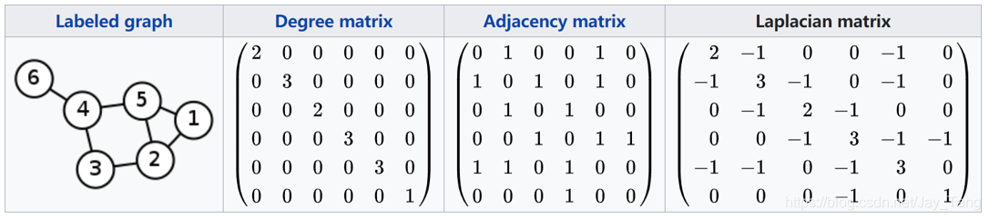
Adjacency $\operatorname{matrix} \mathbf{A}$: The adjacency $\operatorname{matrix} \mathbf{A}$ is a $n \times n$ matrix with $A_{i j}=1$ if $e_{i j} \in E$ and $A_{i j}=0$ if $e_{i j} \notin E$.
-
Degree $\operatorname{matrix} \mathbf{D}$: The degree matrix is a diagonal matrix which contains information about the degree of each vertex (the number of edges attached to each vertex). It is used together with the adjacency matrix to construct the Laplacian matrix of a graph.
-
Laplacian $\operatorname{matrix} \mathbf{L}$: The Laplacian matrix is a matrix representation of a graph, which is defined by $$\mathbf{L} = \mathbf{D} - \mathbf{A} \tag 4$$
-
Symmetric normalized Laplacian $\operatorname{matrix} \mathbf{L}^{sys}$: The normalized graph Laplacian matrix is a mathematical representation of an undirected graph $$ \mathbf{L}^{sys} = \mathbf{D}^{-\frac{1}{2}} \mathbf{L} \mathbf{D}^{-\frac{1}{2}} \tag 5$$
The symmetric normalized graph Laplacian matrix possesses the property of being real symmetric positive semidefinite. With this property, the normalized Laplacian matrix can be factored as
$$\mathbf{L}^{sys}=\mathbf{U} \mathbf{\Lambda} \mathbf{U}^{T} \tag 6$$
where
$$\mathbf{U}=\left[\mathbf{u}_{\mathbf{0}}, \mathbf{u}_{\mathbf{1}}, \cdots, \mathbf{u}_{\mathbf{n}-1}\right] \in \mathbf{R}^{n \times n} \tag 7$$
is the matrix of eigenvectors ordered by eigenvalues and $\mathbf{\Lambda}$ is the diagonal matrix of eigenvalues (spectrum), $\Lambda_{i i}=\lambda_{i}$. The eigenvectors of the normalized Laplacian matrix form an orthonormal space, in mathematical words $\mathbf{U}^{T} \mathbf{U}=\mathbf{I}$.
Graph Fourier transform
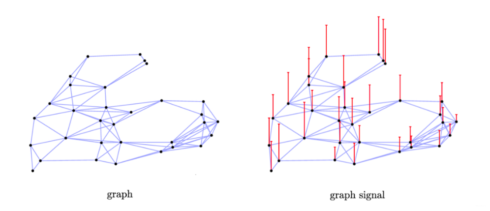
In graph signal processing, a graph signal $\mathbf{x} \in \mathbf{R}^{n}$ is a feature vector of all nodes of a graph where $x_{i}$ is the value of the $i^{t h}$ node.
The graph Fourier transform to a signal $\mathbf{\hat{f}}$ is defined as
$$\mathscr{F}(\mathbf{f})=\mathbf{U}^{T} \mathbf{f} \tag 8$$
and the inverse graph Fourier transform is defined as
$$\mathscr{F}^{-1}(\mathbf{\hat{f}})=\mathbf{U} \mathbf{\hat{f}} \tag 9$$
where $\mathbf{\hat{f}}$ represents the resulted signal from the graph Fourier transform.
Note:
-
$$ \mathbf{\hat{f}} = \left(\begin{array}{c} \hat{f}\left(\lambda_{1}\right) \\ \hat{f}\left(\lambda_{2}\right) \\ \vdots \\ \hat{f}\left(\lambda_{n}\right) \end{array}\right)= \mathbf{U}^{T} \mathbf{f} = \left(\begin{array}{cccc} u_{1}(1) & u_{1}(2) & \ldots & u_{1}(n) \\ u_{2}(1) & u_{2}(2) & \ldots & u_{2}(n) \\ \vdots & \vdots & \ddots & \vdots \\ u_{n}(1) & u_{n}(2) & \ldots & u_{n}(n) \end{array}\right)\left(\begin{array}{c} f(1) \\ f(2) \\ \vdots \\ f(n) \end{array}\right) \tag {10} $$ where $\lambda_i$ are ordered eigenvalues (biggest to smallest), $N$ is the number of nodes.
-
$$\mathbf{\hat{f}}(\lambda_{l})=\sum_{i=1}^{n} \mathbf{f}(i) u_{l}(i) \tag {11}$$
-
$$ \mathbf{f} = \left(\begin{array}{c} f(1) \\ f(2) \\ \vdots \\ f(n) \end{array}\right)= \mathbf{U} \mathbf{\hat{f}} = \left(\begin{array}{cccc} u_{1}(1) & u_{2}(1) & \ldots & u_{n}(1) \\ u_{1}(2) & u_{2}(2) & \ldots & u_{n}(2) \\ \vdots & \vdots & \ddots & \vdots \\ u_{1}(n) & u_{2}(n) & \ldots & u_{n}(n) \end{array}\right)\left(\begin{array}{c} \hat{f}\left(\lambda_{1}\right) \\ \hat{f}\left(\lambda_{2}\right) \\ \vdots \\ \hat{f}\left(\lambda_{n}\right) \end{array}\right) \tag {12} $$
The graph Fourier transform projects the input graph signal to the orthonormal space where the basis is formed by independent eigenvectors ($\mathbf{u}_{\mathbf{0}}, \mathbf{u}_{\mathbf{1}}, \cdots, \mathbf{u}_{\mathbf{n}-1}$) of the normalized graph Laplacian. Elements of the transformed signal $\mathbf{\hat{f}}$ are the coordinates of the graph signal in the new space so that the input signal can be represented as $\mathbf{f}=\sum_{i} \mathbf{\hat{f}}(\lambda_{i}) \mathbf{u}_{i}$ (linear combination of independent eigenvectors, coefficients are entries in vactor $\mathbf{\hat{f}}$), which is exactly the inverse graph Fourier transform.
Now the graph convolution of the input signal $\mathbf{f}$ with a filter $\mathbf{g} \in R^{n}$ is defined as
$$ \begin{aligned} \mathbf{f} *_G \mathbf{g} &=\mathscr{F}^{-1}(\mathscr{F}(\mathbf{f}) \odot \mathscr{F}(\mathbf{g})) \\ &=\mathbf{U}\left(\mathbf{U}^{T} \mathbf{f} \odot \mathbf{U}^{T} \mathbf{g}\right) \\ &=\mathbf{U}\left(\mathbf{\hat f} \odot \mathbf{\hat g}\right) \end{aligned} \tag {13} $$
Note that (13) uses formula from (3)(8)(9).
We know from (10) and (11) that
$$ \mathbf{\hat{f}} = \left(\begin{array}{c} \hat{f}\left(\lambda_{1}\right) \\ \hat{f}\left(\lambda_{2}\right) \\ \vdots \\ \hat{f}\left(\lambda_{n}\right) \end{array}\right) = \left(\begin{array}{c} \mathbf{\hat{f}}(\lambda_{1})=\sum_{i=1}^{n} \mathbf{f}(i) u_{1}(i) \\ \mathbf{\hat{f}}(\lambda_{2})=\sum_{i=1}^{n} \mathbf{f}(i) u_{2}(i) \\ \vdots \\ \mathbf{\hat{f}}(\lambda_{n})=\sum_{i=1}^{n} \mathbf{f}(i) u_{n}(i) \end{array}\right) \tag {14} $$
Therefore, we could write the element-wise product $\mathbf{\hat f} \odot \mathbf{\hat g}$ as
$$ \mathbf{\hat f} \odot \mathbf{\hat g}= \mathbf{\hat g} \odot \mathbf{\hat f}= \mathbf{\hat g} \odot \mathbf{U}^{T} \mathbf{f}= \left(\begin{array}{ccc} \mathbf{\hat g}\left(\lambda_{1}\right) & & \\ & \ddots & \ & & \mathbf{\hat g} \left(\lambda_{n}\right) \end{array}\right) \mathbf{U}^{T} \mathbf{f} \tag {15} $$
If we denote a filter as $\mathbf{g}_{\theta}(\mathbf{\Lambda})=\operatorname{diag}\left(\mathbf{U}^{T} \mathbf{g}\right),$ then the spectral graph convolution is simplified as
$$ \mathbf{f} *_G \mathbf{g} = \mathbf{U g}_{\theta}(\mathbf{\Lambda}) \mathbf{U}^{T} \mathbf{f} \tag {16} $$
Spectral-based ConvGNNs all follow this definition. The key difference lies in the choice of the filter $\mathrm{g}_{\theta}$. In the rest of the post, I list two designs of filter for making a sense of what Spectral Convolutional Neural Network is.
Spectral-based ConvGNNs
Definition:
- (the number of) Input/output channels: dimensionality of node feature vectors.
Spectral Convolutional Neural Network assumes the filter $\mathbf{g}_{\theta}=\Theta_{i, j}^{(k)}$ is a set of learnable parameters and considers graph signals with multiple channels. The graph convolutional layer of Spectral CNN is defined as
$$ \mathbf{H}_{:, j}^{(k)}=\sigma\left(\sum_{i=1}^{f_{k-1}} \mathbf{U} \Theta_{i, j}^{(k)} \mathbf{U}^{T} \mathbf{H}_{:, i}^{(k-1)}\right) \quad\left(j=1,2, \cdots, f_{k}\right) \tag {17} $$
where $k$ is the layer index, $\mathbf{H}^{(k-1)} \in \mathbf{R}^{n \times f_{k-1}}$ is the input graph signal, $\mathbf{H}^{(0)}=\mathbf{X}$ (node feature matrix of a graph), $f_{k-1}$ is the number of input channels and $f_{k}$ is the number of output channels, $\Theta_{i, j}^{(k)}$ is a diagonal matrix filled with learnable parameters.
Due to the eigen-decomposition of the Laplacian matrix, Spectral CNN faces three limitations:
-
Any perturbation to a graph results in a change of eigenbasis.
-
The learned filters are domain dependent, meaning they cannot be applied to a graph with a different structure.
-
Eigen-decomposition requires $O\left(n^{3}\right)$ computational complexity ($n$: the number of nodes).
Naive Design of $\mathbf{g}_{\theta}(\mathbf{\Lambda})$
The naive way is to set $\mathbf{\hat g}(\lambda_l) = \theta_l$, that is,
$$ g_{\theta}(\mathbf{\Lambda})=\left(\begin{array}{ccc} \theta_{1} & & \\ & \ddots & \\ & & \theta_{n} \end{array}\right) \tag {18} $$
Limitations:
-
In each forward-propagation step, we need to calculate the product of the three matrices The amount of calculation is too large especially for relatively large graphs.
-
Convolution kernel does not have Spatial Localization.
-
The number of $\theta_l$ depends on the total number of nodes, which is unacceptable for large graph.
In follow-up works, ChebNet, for example, reduces the computational complexity by making several approximations and simplifications.
Chebyshev Spectral CNN (Recursive formulation for fast filtering)
Polynomial parametrization for localized filters
Limitations mentioned in the last section can be overcome with the use of a polynomial filter, where
$$\mathbf{\hat g}(\lambda_l) = \sum_{i=0}^{K} \theta_{l} \lambda^{l} \tag{19}$$
Written in the matrix format, we have
$$ g_{\theta}(\mathbf{\Lambda})=\left(\begin{array}{ccc} \sum_{i=0}^{K} \theta_{i} \lambda_{1}^{i} & & \\ & \ddots & \ & & \sum_{i=0}^{K} \theta_{i} \lambda_{n}^{i} \end{array}\right)=\sum_{i=0}^{K} \theta_{i} \Lambda^{i} \tag{20} $$
Then, replacing new defined $g_{\theta}(\mathbf{\Lambda})$ in (16), we have
$$\mathbf{f} *_G \mathbf{g} = U (\sum_{i=0}^{K} \theta_{i} \Lambda^{i}) U^{T} \mathbf{f} =\sum_{i=0}^{K} \theta_{i} (U \Lambda^{i} U^{T}) \mathbf{f} =\sum_{i=0}^{K} \theta_{i} L^{i} \mathbf{f} \tag {21}$$
By using polynomial parametrization,
-
Parameters reduce from $n$ to $K+1$.
-
We no longer have to multiply three matrices, but instead we only need to calculate powers of matrix $L$.
-
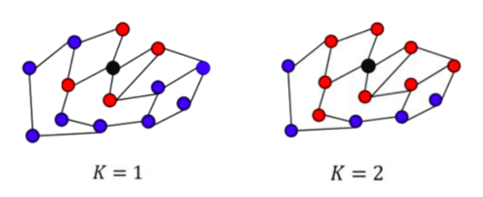
It can be shown that this filter is localized in space (Spatial Localization). In other words, spectral filters represented by $K$th-order polynomials of the Laplacian are exactly K-localized (K-localized means the model is aggregating the information from neighbors within $K$th order, see the figure above).
Chebyshev Spectral CNN (ChebNet)
Chebyshev Spectral CNN (ChebNet) approximates the filter $g_{\theta}(\mathbf{\Lambda})$ by Chebyshev polynomials of the diagonal matrix of eigenvalues, i.e,
$$\mathrm{g}_{\theta}(\mathbf{\Lambda})=\sum_{i=0}^{K} \theta_{i} T_{i}(\tilde{\boldsymbol{\Lambda}}) \tag{22}$$
where
-
$\tilde{\boldsymbol{\Lambda}}=2 \mathbf{\Lambda} / \lambda_{\max }- \mathbf{I}_{\mathbf{n}}$, a diagonal matrix of scaled eigenvalues that lie in $[−1, 1]$.
-
The Chebyshev polynomials are defined recursively by $$T_{i}(\mathbf{f})=2 \mathbf{f} T_{i-1}(\mathbf{f})-T_{i-2}(\mathbf{f}) \tag{23}$$ with $T_{0}(\mathbf{f})=1$ and $T_{1}(\mathbf{f})=\mathbf{f}$.
As a result, the convolution of a graph signal $\mathbf{f}$ with the defined filter $\mathrm{g}_{\theta}(\mathbf{\Lambda})$ is $$ \mathbf{f} *_{G} \mathbf{g}_{\theta}=\mathbf{U}\left(\sum_{i=0}^{K} \theta_{i} T_{i}(\tilde{\boldsymbol{\Lambda}})\right) \mathbf{U}^{T} \mathbf{f} \tag{24} $$
Denote scaled Laplacian $\tilde{\mathbf{L}}$ as
$$\tilde{\mathbf{L}}=2 \mathbf{L} / \lambda_{\max }-\mathbf{I}_{\mathbf{n}} \tag {25}$$
Then by induction on $i$ and using (21), the following equation holds:
$$T_{i}(\tilde{\mathbf{L}})=\mathbf{U} T_{i}(\tilde{\boldsymbol{\Lambda}}) \mathbf{U}^{T} \tag {26}$$
Then finally ChebNet takes the following form:
$$ \mathbf{f} *_{G} \mathbf{g}_{\theta}=\sum_{i=0}^{K} \theta_{i} T_{i}(\tilde{\mathbf{L}}) \mathbf{f} \tag {27} $$
The benefits of ChebNet is similar to those of polynomial parametrization mentioned above.
Comparison between spectral and spatial models
Spectral models have a theoretical foundation in graph signal processing. By designing new graph signal filters, one can build new ConvGNNs. However, spatial models are preferred over spectral models due to efficiency, generality, and flexibility issues.
First, spectral models are less efficient than spatial models. Spectral models either need to perform eigenvector computation or handle the whole graph at the same time. Spatial models are more scalable to large graphs as they directly perform convolutions in the graph domain via information propagation. The computation can be performed in a batch of nodes instead of the whole graph.
Second, spectral models which rely on a graph Fourier basis generalize poorly to new graphs. They assume a fixed graph. Any perturbations to a graph would result in a change of eigenbasis. Spatial-based models, on the other hand, perform graph convolutions locally on each node where weights can be easily shared across different locations and structures.
Third, spectral-based models are limited to operate on undirected graphs. Spatial-based models are more flexible to handle multi-source graph inputs such as edge inputs, directed graphs, signed graphs, and heterogeneous graphs, because these graph inputs can be incorporated into the aggregation function easily.
Reference:
- Introduction to the Fourier Transform: http://www.thefouriertransform.com/#introduction
- Degree Matrix: https://en.wikipedia.org/wiki/Degree_matrix
- Introduction to Graph Signal Processing: https://link.springer.com/chapter/10.1007/978-3-030-03574-7_1
- Convolution Theorem: https://www.sciencedirect.com/topics/engineering/convolution-theorem
- The Convolution Theorem with Application Examples: https://dspillustrations.com/pages/posts/misc/the-convolution-theorem-and-application-examples.html
Paper:
- A Comprehensive Survey on Graph Neural Networks: https://arxiv.org/pdf/1901.00596.pdf
- Spectral Networks and Deep Locally Connected Networks on Graphs https://arxiv.org/pdf/1312.6203.pdf
- Spectral Networks and Deep Locally Connected Networks on Graphs: https://arxiv.org/pdf/1312.6203.pdf
- Convolutional Neural Networks on Graphs with Fast Localized Spectral Filtering: https://arxiv.org/pdf/1606.09375.pdf