Note
This is the second post of the Graph Neural Networks (GNNs) series.
Convolutional graph neural networks (ConvGNNs)
Convolutional graph neural networks (ConvGNNs) generalize the operation of convolution from grid data to graph data. The main idea is to generate a node $v$’s representation by aggregating its own features $\mathbf{x}_{v}$ and neighbors’ features $\mathbf{x}_{u}$, where $u \in N(v)$. Different from RecGNNs, ConvGNNs stack fixed number of multiple graph convolutional layers with different weights to extract high-level node representations.
ConvGNNs fall into two categories:
-
spatial-based GCN: Spatial-based approaches inherit ideas from RecGNNs to define graph convolutions by information propagation.
-
spectral-based GCN: Spectral based approaches define graph convolutions by introducing filters from the perspective of graph signal processing where the graph convolutional operation is interpreted as removing noises from graph signals.
Spatial-based methods have developed rapidly recently due to its attractive efficiency, flexibility, and generality. In this post, we mainly focus on spatial-based GCN and leave spectral-based GCN to the next post. Let’s get started.
GCN Framework
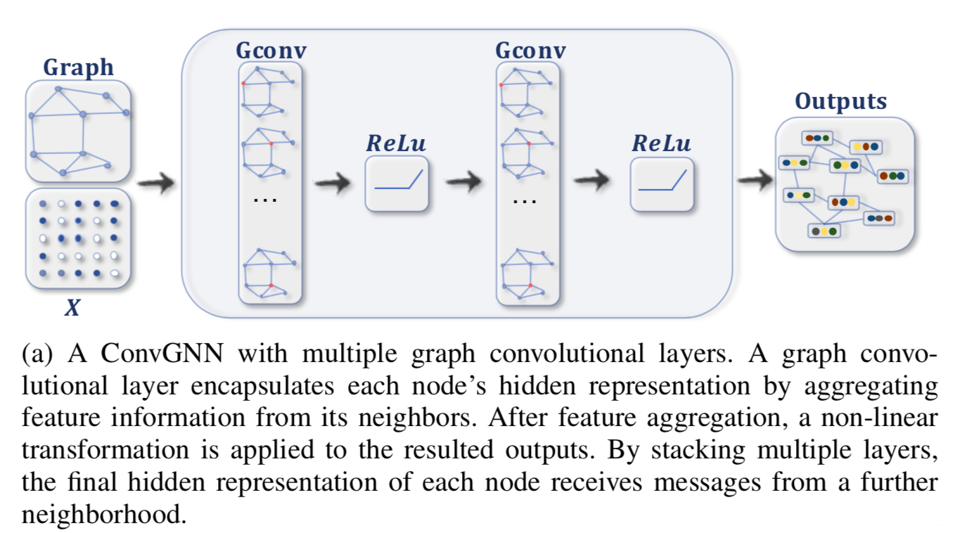
As shown in the figure above, the input of GCN is the entire graph. In each convolution layer, a convolution operation is performed on the neighbors of each node, and the center node representation is updated with the result of the convolution. Then an activation function such as ReLU is used before going through the next layer of convolution layer. The above process continues until the number of layers reaches the expected depth (a hyper-parameter).
GCN v.s. RecGNN
The main difference between GCN and RecGNN is that each convolutional layer of GCN has unique weights, and, on the other hand, in RecGNN the weights of each layer are shared.
What is Convolution
In mathematics, convolution is a mathematical operation on two functions $f$ and $g$ that produces a third function $(f∗g)$ expressing how the shape of one is modified by the other.
The term convolution is defined as the integral of the product of the two functions after one is reversed and shifted. The mathematical definition is the following:
$$ \begin{array}{c} (f * g)(t)=\int_{-\infty}^{\infty} f(\tau) g(t-\tau) \quad (\text {continuous}) \\ (f * g)(t)=\sum_{\tau=-\infty}^{\infty} f(\tau) g(t-\tau) \quad(\text {discrete}) \end{array} $$
The convolution formula can be described as a weighted average of the function $f(\tau)$ at the moment $t$ where the weighting is given by $g(-\tau)$ simply shifted by amount $t$. As $t$ changes, the weighting function emphasizes different parts of the input function.

As the figure shown above, the filter is moved over by one pixel and this process is repeated until all of the possible locations in the image are filtered. At each step, the convolution takes the weighted average of pixel values of the center pixel along with its neighbors. Since the center pixel is changing at each time step, the convolution is emphasizing on different parts of the image.
Spatial-based ConvGNNs
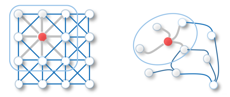
Analogous to the convolutional operation of a conventional CNN on an image, spatial-based methods define graph convolutions based on a node’s spatial relations.
Images can be considered as a special form of graph with each pixel representing a node. Each pixel is directly connected to its nearby pixels, as illustrated in the figure above (left). A filter is applied to a $3 \times 3$ patch by taking the weighted average of pixel values of the central node and its neighbors across each channel.
Similarly, the spatial-based graph convolutions convolve the central node’s representation with its neighbors’ representations to derive the updated representation for the central node. From another perspective, spatial-based ConvGNNs share the same idea of information propagation/message passing with RecGNNs. The spatial graph convolutional operation essentially propagates node information along edges.
Message Passing Neural Network (MPNN)
Introduction to MPNN
Message Passing Neural Network (MPNN) outlines a general framework of spatial-based ConvGNNs (It is not actually a model). It treats graph convolutions as a message passing process in which information can be passed from one node to another along edges directly. MPNN runs K-step message passing iterations to let information propagate further. The message passing function (namely the spatial graph convolution) is defined as
$$ \mathbf{h}_{v}^{(k)}=U_{k}\left(\mathbf{h}_{v}^{(k-1)}, \sum_{u \in N(v)} M_{k}\left(\mathbf{h}_{v}^{(k-1)}, \mathbf{h}_{u}^{(k-1)}, \mathbf{x}_{(v,u)}\right)\right) \tag 1 $$
or we can write it separately as:
$$ \begin{array} \mathbf{m}_v^{k} = \sum_{u \in N(v)} M_{k}\left(\mathbf{h}_{v}^{(k-1)}, \mathbf{h}_{u}^{(k-1)}, \mathbf{x}_{(v,u)}\right) \ \mathbf{h}_{v}^{(k)}=U_{k}\left(\mathbf{h}_{v}^{(k-1)}, \mathbf{m}_v^{k}\right) \tag 2\ \end{array} $$
Note:
- $\mathbf{m}_v^{k}$ represents messages at node $v$ at time step $k$;
- $\mathbf{h}_{v}^{(0)}=\mathbf{x}_{v}$;
- $U_{k}(\cdot)$ and $M_{k}(\cdot)$ are functions with learnable parameters.
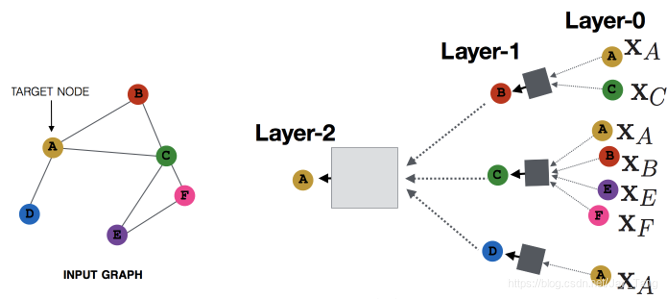
- From (2), we see that MPNN has two main steps: information passing and state update. $M_{k}(\cdot)$ is the function for information passing and $U_{k}(\cdot)$ is the function for state update.
- The formula can be interpreted as each node first collects information from neighbors and then updates its own hidden state.
For example, here is an illustration of updating node $A$:
After deriving the hidden representations of each node, $\mathbf{h}_{v}^{(K)}$ can be passed to an output layer to perform node-level prediction tasks or to a readout function to perform graph-level prediction tasks. The readout function generates a representation of the entire graph based on node hidden representations (I will talk about readout function in a later post). It is generally defined as $$ \mathbf{h}_{G}=R\left(\mathbf{h}_{v}^{(K)} \mid v \in G\right) $$ where $R(\cdot)$ represents the readout function with learnable parameters, and $\mathbf{h}_{G}$ is a representation of the entire graph.
Note that MPNN can cover many existing GNNs by assuming different forms of $U_{k}(\cdot), M_{k}(\cdot),$ and $R(\cdot)$.
Shortage of the MPNN framework
The shortage of MPNN is that it convolves on the entire graph, which means that all nodes must be put into the memory to perform the convolution operation. But for large-scale graph, the convolution operation on the entire graph is not realistic. In the next section, I’m going to introduce a model (GraphSAGE) to overcome this problem.
GraphSAGE (SAmple and aggreGatE)
Overview of GraphSAGE
As the number of neighbors of a node can vary from one to a thousand or even more, it is inefficient to take the full size of a node’s neighborhood. GraphSage adopts sampling to obtain a fixed number of neighbors for each node. It performs graph convolutions by
$$ \mathbf{h}_{v}^{(k)}=\sigma(\mathbf{W}^{(k)} \cdot f_{k}\left(\mathbf{h}_{v}^{(k-1)},\left{\mathbf{h}_{u}^{(k-1)}, \forall u \in S_{\mathcal{N}(v)}\right}\right) $$
where $\mathbf{h}_{v}^{(0)}=\mathbf{x}_{v}, f_{k}(\cdot)$ is an aggregation function, $S_{\mathcal{N}(v)}$ is a random sample of the node $v$ ’s neighbors. The aggregation function should be invariant to the permutations of node orderings such as a mean, sum or max function.
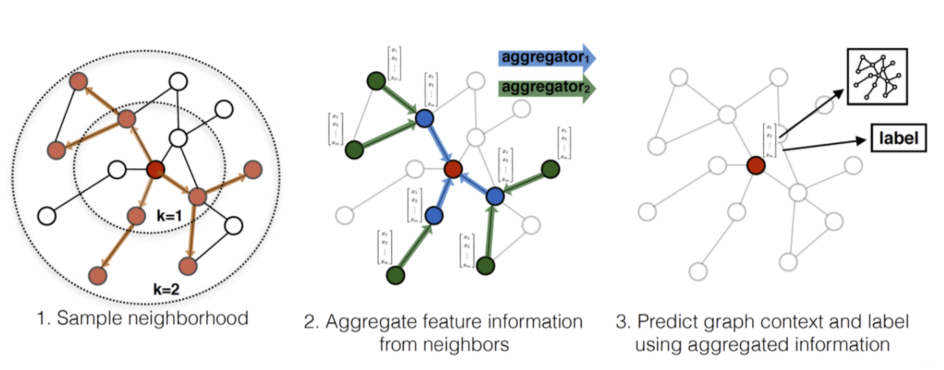
Specifically, the sampling process in GraphSage is divided into three steps (corespond to the figure above):
-
First, several nodes are randomly sampled in the graph. Then for each node, they uniformly sample a fixed-size set of neighbors, instead of using full neighborhood sets. These fixed-size of neighbors are uniformly drawn from all possible neighbors, and they draw different uniform samples at each iteration. Here, neighbors are not necessarily first-order neighbors, but also second-order.
-
Update sampled node’s information by aggregating the information of neighbor nodes through some aggregate functions.
-
Calculate the loss at the sampled node. If it is an unsupervised task, we hope that the neighborhood nodes on the graph share similar node representations; if it is a supervised task, we can calculate the loss based on the task label of the specific node.
Aggregator Fuctions
Ideally, an aggregator function would be invariant to permutations of its inputs. This property of the aggregation function ensures that a neural network model canbe trained and applied to arbitrarily ordered node neighborhood feature sets. In the paper, they examed three aggregation functions: Mean Aggregator, LSTM Aggretator, Pooling Aggretator.
Mean Aggregator: Their first examed aggregator function is the mean operator, where we simply take the elementwise mean of the vectors in $\left{\mathbf{h}{u}^{(k-1)}, \forall u \in S{\mathcal{N}(v)}\right}$. That is:
$$ \mathbf{h}_{v}^{(k)}=\sigma(\mathbf{W}^{(k)} \cdot \text{MEAN}\left({\mathbf{h}_{v}^{(k-1)}} \cup \left{\mathbf{h}_{u}^{(k-1)}, \forall u \in S_{\mathcal{N}(v)}\right}\right) $$
LSTM Aggregator: Compared to the mean aggregator, LSTMs have the advantage of larger expressive capability. However, it is important to note that LSTMs are not permutation invariant, since they process their inputs in a sequential manner. They adapt LSTMs to operate on an unordered set by simply applying the LSTMs to a random permutation of the node’s neighbors.
Pooling Aggregator: each neighbor’s vector is independently fed through a fully-connected neural network; following this transformation, an elementwise max-pooling operation is applied to aggregate information across the neighbor set:
$$ \text {AGGREGATE}_{k}^{\text {pool}}=\max \left({\sigma\left(\mathbf{W}_{\text {pool }} \mathbf{h}_{u}^{(k)}+\mathbf{b}\right), \forall u \in S_{\mathcal{N}(v)}}\right) $$
where $\max$ denotes the element-wise max operator and $\sigma$ is a nonlinear activation function.
The key point of the aggregstion function is that it can handle input with vaiable length.
PATCHY-SAN
Another distinct line of works achieve weight sharing across different locations by ranking a node’s neighbors based on certain criteria and associating each ranking with a learnable weight.
Overview of PATCHY-SAN
Definitions:
-
Node degree: The degree of a node is the number of edges connected to the node.
-
Graph labelings: Graph labelings are essentially node scores which can be derived by node degree, centrality, and Weisfeiler-Lehman algorithm (a procedure for partitioning the vertices of a graph. It is also known as color refinement).
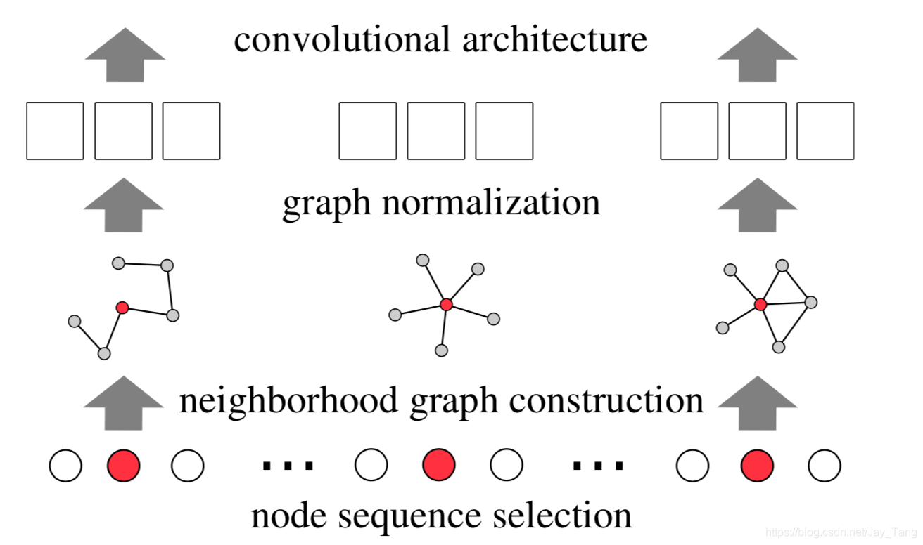
PATCHY-SAN orders neighbors of each node according to their graph labelings and selects the top $\omega$ neighbors. As each node now has a fixed number of ordered neighbors, graph-structured data can be converted into grid-structured data. PATCHY-SAN applies a standard 1D convolutional filter to aggregate neighborhood feature information where the order of the filter’s weights corresponds to the order of a node’s neighbors. The ranking criterion of PATCHY-SAN only considers graph structures.
Two problems considered in PATCHY-SAN
-
Given a collection of graphs, learn a function that can be used for classification and regression problems on unseen graphs.
-
Given a large graph, learn graph representations that can be used to infer unseen graph properties such as node types and missing edges.
Steps of PATCHY-SAN
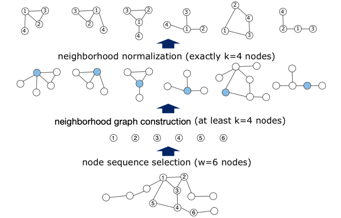
PATCHY-SAN solves the above two problems through the following three steps:
-
Node Squenece Selection: Specify an order in the graph for each node through some human-defined rules (e.x., a node with a large degree has a high score). Then take the first $\omega$ nodes as the representative of the whole graph. If the number of nodes is smaller than $\omega$, empty nodes should be used for padding.
-
Neighborhood graph construction: Take the nodes selected in the previous step as the center. Get their neighbors (can be first-order or second-order), which form $\omega$ cliques. Sort the neighbors in each clique according to the node ranking obtained in the previous step, and then take the first $k$ neighbors and arrange them in order, that is, form $\omega$ ordered cliques. If the number of nodes is smaller than $k$, empty nodes should be used for padding.
-
Graph Normalization: The normalization imposes an order on the nodes of the neighborhood graph so as to map from the unordered graph space to a vector space with a linear order. According to the graph labeling in each clique, all cliques can be converted into a fixed-length sequence $(k+1)$, including the center node. Then they can be concatenated according to the order of the center nodes to obtain a sequence with length of $\omega \cdot (k +1)$, which represents the entire graph. In this way, we can directly use the 1D convolution to model the sequence.
Reference:
- Convolution: https://en.wikipedia.org/wiki/Convolution
- From graph to graph convolution (2): https://www.cnblogs.com/SivilTaram/p/graph_neural_network_2.html
- http://www.matlog.net/icml2016_slides.pdf
Paper
- A Comprehensive Survey on Graph Neural Networks: https://arxiv.org/pdf/1901.00596.pdf
- Inductive Representation Learning on Large Graphs: https://arxiv.org/pdf/1706.02216.pdf
- Neural Message Passing for Quantum Chemistry: https://arxiv.org/pdf/1704.01212.pdf
- Learning Convolutional Neural Networks for Graphs: https://arxiv.org/pdf/1605.05273.pdf