Generative model v.s. Discriminative model:
Examples:
- Generative model: Naive Bayes, HMM, VAE, GAN.
- Discriminative model:Logistic Regression, CRF.
Objective function:
- Generative model: $max \ p \ (x,y)$
- Discriminative model:$max \ p \ (y \ |\ x)$
Difference:
- Generative model: We first assume a distribution of the data in the consideration of computation efficiency and features of the data. Next, the model will learn the parameters of distribution of the data. Then, we can use the model to generate new data. (e.g. generate new data from a normal distribution.)
- Discriminative model: The only purpose is to classify, that is, to tell the difference. As long as it can find a way to tell the difference, it doesn’t need to learn anything else.
Relation:
- Generative model: $p\ (x,y) = p\ (y \ |\ x) \ p(y)$, it has a prior term $p(y)$.
- Discriminative model:$p\ (y \ |\ x)$
- Both models can do classification problems, but discriminative model can do classification problems only. Usually, for classification problems, discriminative model performs better. On the other hand, if we have limited data, generative model might perform better (since it has a prior term, which plays the role of a regularization).
Logistic regression
Formula:
$$ \sigma(x) = \frac{1}{1 + e^{-w^Tx}}$$
Derivative formula:
- $\sigma'(x) = \sigma(x)(1-\sigma(x))$
Logistic Regression does not have analytic solutions and we need to use iterative optimization to find a solution recursively.
It spends a lot of computational power to calculate $e^x$ because of floating points. In most code implementation, people will pre-calculate values and then do approximate with a new $x$ comes.
Derivation of Logistic Regression
$$ \begin{aligned} p(y | x, w, b) &=p(y=1 | x, w, b)^{y}[1-p(y=1 | x, w, b)]^{1-y} \\ \hat{w}_{MLE}, \hat{b}_{MLE} &= \argmax_{w, b} \prod_{i=1}^{n} p\left(y_{i} | x_{i}, w, b\right) \\ &=\argmax_{w, b} \sum_{i=1}^{n} \log p\left(y_{i} | x_{i}, w, b\right) \\ &=\argmin_{w, b}-\sum_{i=1}^{n} \log p\left(y_{i} | x_{i}, w, b\right) \\ &=\argmin_{w, b}-\sum_{i=1}^{n} \log \left[p\left(y_{i}\right) | x_{i}, w, b\right)^{y_{i}}\left[1-p\left(y_{i}=1 | x_{2}, w, b\right)^{-y_{i}}\right] \\ &=\argmin_{w, b}-\sum_{i=1}^{n} y_{i} \log p\left(y_{i}=1 | x_{i}, w, b\right)+\left(1-y_{i}\right) \log \left[1-p\left(y_{i}=1 | x_{i} w, b\right)\right] \\ &=\argmin_{w, b} L \ \frac{\partial L}{\partial b} &= -\sum_{i=1}^{n}\left(y_{i} \cdot \frac{\sigma (w^{T}x_{i} + b) \cdot [1-\sigma (w^{T}x_{i} + b)]}{\sigma(w^{T}x_i+b)}-(1-y_i) \cdot \frac{-\sigma\left(w^{T} x_{i}+b\right)\left[1-\sigma\left(w^{T} x_{i}+b\right)\right]}{1-\sigma\left(w ^{T}x_i+b\right)}\right] & \\ &=-\sum_{i=1}^{n}\left(y_{i}\left[1-\sigma\left(w^{T} x_{i}+b\right)\right]-\left(1-y_{i}\right)\sigma(w^{T}x_i + b) \right) \\ &= \sum_{i=1}^{n}\left(\sigma\left(w^{T} x_{i}+b\right)-y_{i}\right)\ \frac{\partial L}{\partial w}&=\sum_{i=1}^{n}\left(\sigma\left(w^{T} x_{i}+b\right)-y_{i}\right) \cdot x_{i} \end{aligned} $$
Gradient:
True gradient: The true gradient of the population.
Empirical gradient: Use sample gradient to approximate true gradient.
- SGD, approximate bad. Asymptotically converge to true gradient.
- GD, approximate good.
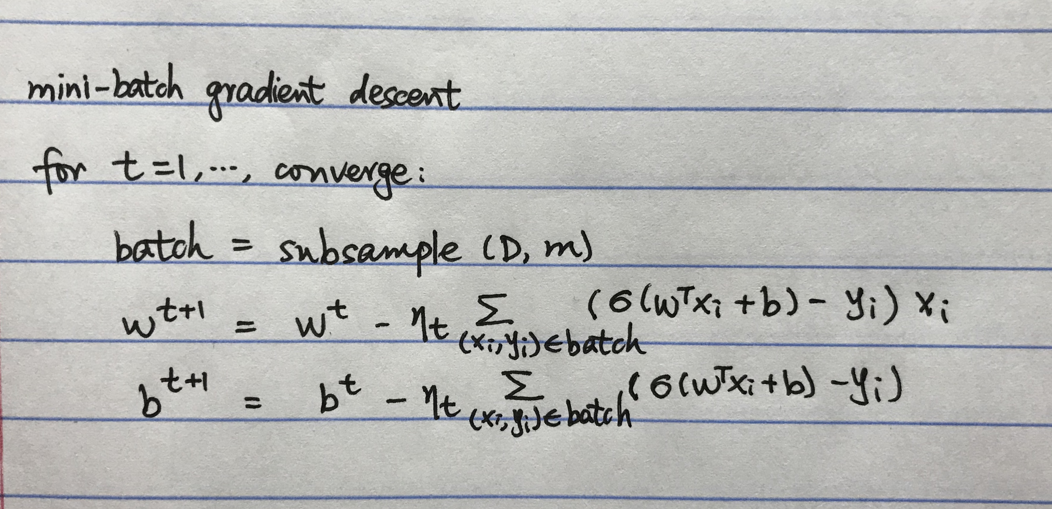
- mini-batch DG, middle.
For smooth optimization, we can use gradient descent.
For non-smooth optimization, we can use coordinate descent (e.g. L1).
Mini-Batch Gradient Descent for Logistic Regression
Way to prevent overfitting:
- More data.
- Regularization.
- Ensemble models.
- Less complicate models.
- Less Feature.
- Add noise (e.g. Dropout)
L1 regularization
L1: Feature Selection, PCA: Features changed.
Why prefer sparsity:
- reduce dimension, then less computation.
- Higher interpretability.
Problem of L1:
- Group Effect: If there is collinearity in features, L1 will randomly choose one from each group. Therefore, the best feature in each group might not be selected.
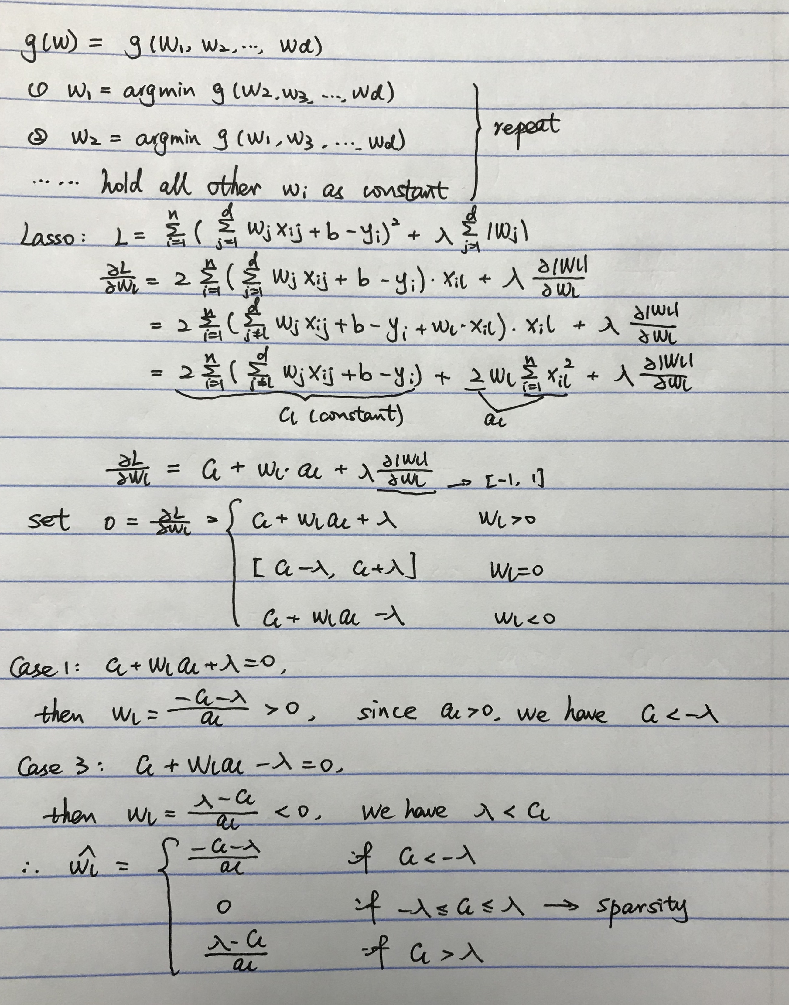
Coordinate Descent for Lasso
-
Intuition: If we are at a point $x$ such that $f(x)$ is minimized along each coordinate axis, then we find a global minimizer.
-
step of Coordinate Descent: Note that we don’t need a learning rate here since we are finding the optimum values.
Large eigenvalue by co-linear columns
If a matrix 𝐴 has an eigenvalue $\lambda$, then $A^{-1}$ have an eigenvalue $\frac{1}{\lambda}$
$$A\mathbf{v} = \lambda\mathbf{v} \implies A^{-1}A\mathbf{v} = \lambda A^{-1}\mathbf{v}\implies A^{-1}\mathbf{v} = \frac{1}{\lambda}\mathbf{v}$$
If a matrix $A = X^{T}X$ has a very small eigenvalue, then its inverse $(X^{T}X)^{-1}$ has a very big eigenvalue. We know that the formula for $\beta$ is $$\hat \beta = (X^{T}X)^{-1}X^{T}y$$
If we plug in $y = X\beta^{} + \epsilon$, then $$\hat \beta = \beta^{} + (X^{T}X)^{-1}X^{T}\epsilon$$
Multiplying the noise by $(X^{T}X)^{-1}$ has the potential to blow up the noise. This is called “noise amplification”. If we set the error term $\epsilon$ to zero, then there is no noise to amplify. Hence there are no problems with the huge eigenvalues of $(X^{T}X)^{-1}$, and we still recover the correct answer. But even a little bit of error, and this goes out the window.
If we now add some regularization (aka weight decay), then $$\hat \beta = (X^{T}X + \lambda I)^{-1}X^{T}y$$
Adding a small multiple of the identity to $X^{T}X$ barely changes the large eigenvalues, but it drastically changes the smallest eigenvalue – it increases it to $\lambda$. Thus in the inverse, the largest eigenvalue will be at most $\frac{1}{\lambda}$.
Building Models with prior knowledge (put relation into models via regularization):
- model + $\lambda \cdot$ Regularization
- Constraint optimization
- Probabilistic model (e.g. Probabilistic Graph Model (PGM))