Note
This post is the second part of overall summarization of the competition. The first half is here.
Noteworthy ideas in 1st place solution
Idea
First step:
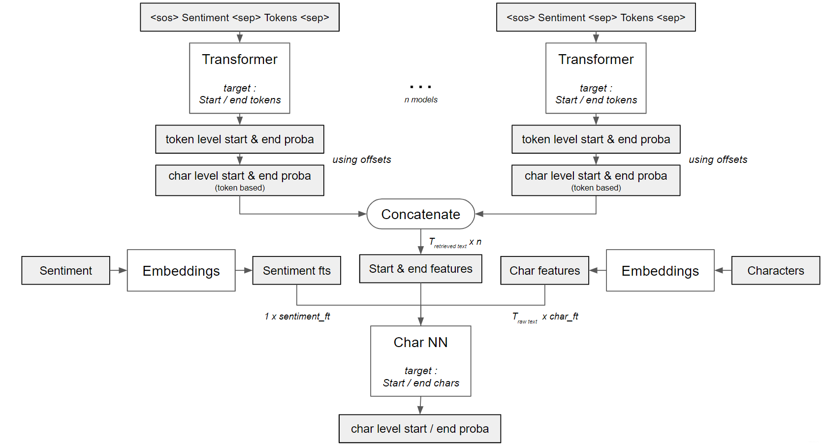
Use transformers to extract token level start and end probabilities.
Second step:
Feed these probabilities to a character level model. This step gives the team a huge improve on the final score since it handled the “noise” in the data properly.
Last step:
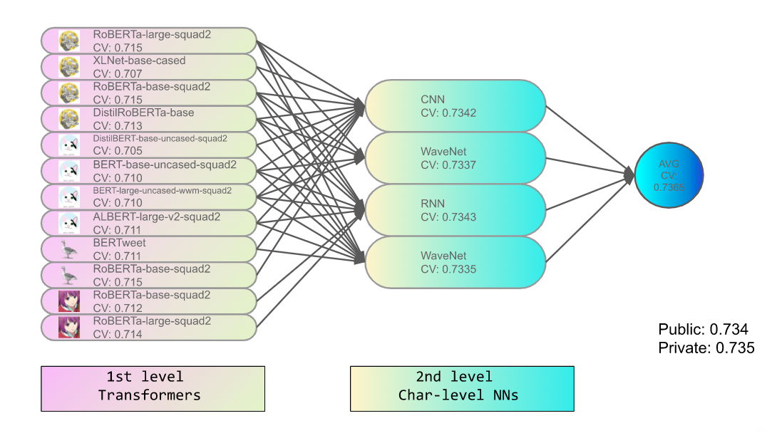
Ensemble.
Second level models Architectures
The following three Char-NN architectures uses character-level probabilities as input. The first level models output token-level probabilities and the following code convert token-level probabilities to character-level probabilities. The idea in the following cide is to assigning each character the probability of the corresponding token.
def token_level_to_char_level(text, offsets, preds):
    probas_char = np.zeros(len(text))
    for i, offset in enumerate(offsets):
        if offset[0] or offset[1]: # remove padding and sentiment
            probas_char[offset[0]:offset[1]] = preds[i]

    return probas_char
Things you need to know for nn.Embedding
The following architectures all train the embedding from scratch. Here we want to shortly discuss how nn.Embedding works.
nn.Embedding holds a Tensor of dimension (vocab_size, vector_size), i.e., of (the size of the vocabulary, the dimension of each vector embedding), and a method that does the lookup. When you create an embedding layer, the Tensor is initialised randomly.
You can also add pretrained weights with the command nn.Embedding.from_pretrained(weight).
Architecture 1: RNN
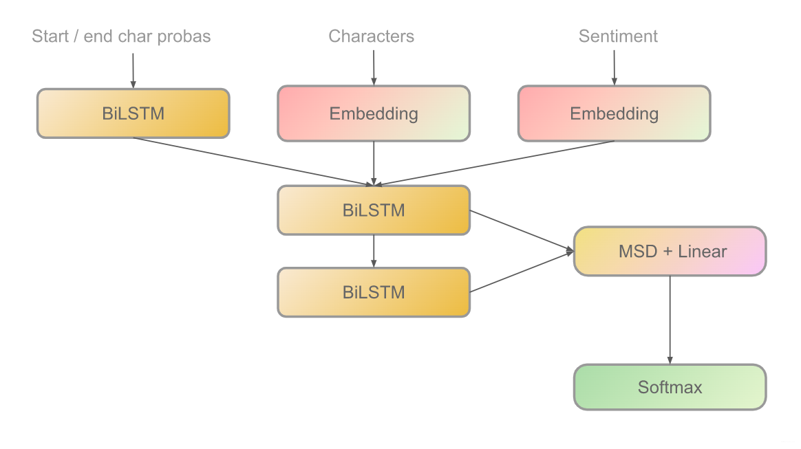
In the following, the parameter len_voc is calculated by
tokenizer.fit_on_texts(df_train['text'].values)
len_voc = len(tokenizer.word_index) + 1
Compare the following code with the figure above.
class TweetCharModel(nn.Module):
    # check the config in the original code post
    def __init__(self, len_voc, use_msd=True,
                 embed_dim=64, lstm_dim=64, char_embed_dim=32, sent_embed_dim=32, ft_lstm_dim=32, n_models=1):
        super().__init__()
        self.use_msd = use_msd

        self.char_embeddings = nn.Embedding(len_voc, char_embed_dim)
        self.sentiment_embeddings = nn.Embedding(3, sent_embed_dim) # 3 sentiments

        self.proba_lstm = nn.LSTM(n_models * 2, ft_lstm_dim, batch_first=True, bidirectional=True)

        self.lstm = nn.LSTM(char_embed_dim + ft_lstm_dim * 2 + sent_embed_dim, lstm_dim, batch_first=True, bidirectional=True)
        self.lstm2 = nn.LSTM(lstm_dim * 2, lstm_dim, batch_first=True, bidirectional=True)

        self.logits = nn.Sequential(
            nn.Linear(lstm_dim *  4, lstm_dim),
            nn.ReLU(),
            nn.Linear(lstm_dim, 2))

        self.high_dropout = nn.Dropout(p=0.5)

    def forward(self, tokens, sentiment, start_probas, end_probas):
        bs, T = tokens.size()

        probas = torch.cat([start_probas, end_probas], -1)
        probas_fts, _ = self.proba_lstm(probas)

        char_fts = self.char_embeddings(tokens)

        sentiment_fts = self.sentiment_embeddings(sentiment).view(bs, 1, -1)
        sentiment_fts = sentiment_fts.repeat((1, T, 1))

        features = torch.cat([char_fts, sentiment_fts, probas_fts], -1)
        features, _ = self.lstm(features)
        features2, _ = self.lstm2(features)

        features = torch.cat([features, features2], -1)

        # Multi-sample dropout (MSD)
        if self.use_msd and self.training:
            logits = torch.mean(
                torch.stack(
                    [self.logits(self.high_dropout(features)) for _ in range(5)],
                    dim=0),
                dim=0)
        else:
            logits = self.logits(features)

        start_logits, end_logits = logits[:, :, 0], logits[:, :, 1]

        return start_logits, end_logits
Architecture 2: CNN
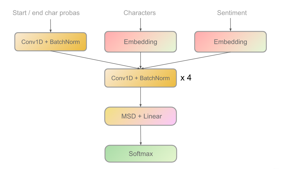
class ConvBlock(nn.Module):
    # check the config in the original code post
    def __init__(self, in_channels, out_channels, kernel_size=3, stride=1, dilation=1, padding="same", use_bn=True):
        super().__init__()
        if padding == "same":
            padding = kernel_size // 2 * dilation

        if use_bn:
            self.conv = nn.Sequential(
                nn.Conv1d(in_channels, out_channels, kernel_size, padding=padding, stride=stride, dilation=dilation),
                nn.BatchNorm1d(out_channels),
                nn.ReLU())
        else:
            self.conv = nn.Sequential(
                nn.Conv1d(in_channels, out_channels, kernel_size, padding=padding, stride=stride, dilation=dilation),
                nn.ReLU())

    def forward(self, x):
        return self.conv(x)

class TweetCharModel(nn.Module):
    def __init__(self, len_voc, use_msd=True,
                 cnn_dim=64, char_embed_dim=32, sent_embed_dim=32, proba_cnn_dim=32, n_models=1, kernel_size=3, use_bn=False):
        super().__init__()
        self.use_msd = use_msd

        self.char_embeddings = nn.Embedding(len_voc, char_embed_dim)
        self.sentiment_embeddings = nn.Embedding(3, sent_embed_dim)

        self.probas_cnn = ConvBlock(n_models * 2, proba_cnn_dim, kernel_size=kernel_size, use_bn=use_bn)

        self.cnn = nn.Sequential(
            ConvBlock(char_embed_dim + sent_embed_dim + proba_cnn_dim, cnn_dim, kernel_size=kernel_size, use_bn=use_bn),
            ConvBlock(cnn_dim, cnn_dim * 2, kernel_size=kernel_size, use_bn=use_bn),
            ConvBlock(cnn_dim * 2 , cnn_dim * 4, kernel_size=kernel_size, use_bn=use_bn),
            ConvBlock(cnn_dim * 4, cnn_dim * 8, kernel_size=kernel_size, use_bn=use_bn))

        self.logits = nn.Sequential(
            nn.Linear(cnn_dim * 8, cnn_dim),
            nn.ReLU(),
            nn.Linear(cnn_dim, 2))

        self.high_dropout = nn.Dropout(p=0.5)

    def forward(self, tokens, sentiment, start_probas, end_probas):
        bs, T = tokens.size()

        probas = torch.cat([start_probas, end_probas], -1).permute(0, 2, 1)
        probas_fts = self.probas_cnn(probas).permute(0, 2, 1)

        char_fts = self.char_embeddings(tokens)

        sentiment_fts = self.sentiment_embeddings(sentiment).view(bs, 1, -1)
        sentiment_fts = sentiment_fts.repeat((1, T, 1))

        x = torch.cat([char_fts, sentiment_fts, probas_fts], -1).permute(0, 2, 1)

        features = self.cnn(x).permute(0, 2, 1) # [Bs x T x nb_ft]

        if self.use_msd and self.training:
            logits = torch.mean(
                torch.stack(
                    [self.logits(self.high_dropout(features)) for _ in range(5)],
                    dim=0),
                dim=0)
        else:
            logits = self.logits(features)

        start_logits, end_logits = logits[:, :, 0], logits[:, :, 1]

        return start_logits, end_logits
Architecture 3: WaveNet
This is a model architecture from another competition, so I ignore the author’s detail here. I attached the source code in the reference.
stacking ensemble
Their solution has no post-processing and just modeling. The following is the idea how they did the final ensemble.
Noteworthy ideas in 2nd place solution
Ensemble
- Using two different seeds (seed averaging):
RoBERTa Base 11th layer + RoBERTa Large 23th layer + RoBERTa Base MSD + RoBERTa Large MSD
$4$ models $\times$ $2$ seeds = Total $8$ models
Post-processing on the extra space
I attached the pp in the reference. I tried out this pp and it raised my rank to around $20$th.
Reranking-model training (Create multi candidates and choose best one)
What is re-ranking
Their model can predict not only a top-$1$ selected_text candidate but also top-$n$ candidates. So re-ranking means that they re-score these top-$n$ candidate.
Why re-ranking
“I calculated the upper bound jaccard score of top-5 candidates in the validation set and that was 0.87-0.88. (If I choose only top-1, the score is only 0.71-0.72.)
So I realized that there is a huge room for improving score by re-ranking. In fact, in the field of question answering (similar to this task), the re-ranking approach is developed.”
How to re-rank
To re-rank candidates, they used two score.
First one is based on start & end value(after applying softmax) from base-model. Second one is a predicted jaccard score using re-ranking model.
Re-ranking model
Build a second level model on top of previous model.
- input: triple (sentiment, tweet, candidate)
- predict: jaccard score
The way they pass the tuple (sentiment, tweet, candidate) to the model is
tweet_candidate = TOKENIZER.encode(str(tweet) + "  " + str(candidate))
token_ids = [0] + [sentiment] + [2] + [2] + tweet_candidate.ids + [2]
In concrete, they calculated top-$5$ candidates in training and validation set and memorize their jaccard score.
They use a simple roberta-base model to predict jaccard score using MSELoss().
Final re-ranking score
Finally, candidates are re-ranked using this score.
(start value + end value) * 0.5 + predicted jaccard score
Here, start and end value means logits calculated by the base model (i.e. start and end position logits after softmax function). This part of the code is under the reference section.
sequence bucketing (dynamic padding)
Team:"inference time speed up x2 and surprisingly got a better result than not using."
In RNNs, the input sequences are often all padded to the same length by doing something along the lines of this:
x_train = pad_sequences(x_train, maxlen=MAX_LEN)
This is suboptimal because when iterating over the dataset in batches, there will be some batches where the length of all samples is smaller than MAX_LEN. So there will be tokens which are zero everywhere in the batch but are still processed by the RNN. Using sequence bucketing, we can speed this up by dynamically padding every batch to the maximum sequence length which occurs in that batch. Or to e.g. the $95$th percentile of lengths in that batch.
class RerankingCollate:
    def __init__(self):
        self.CONFIG = {}
        self.CONFIG['BUCKET'] = True
        self.CONFIG['MAX_LEN'] = MAX_LEN

    def __call__(self, batch):
        out = {
                'orig_tweet'        : [],
                'sentiment'         : [],
                'orig_selected'     : [],
                'jaccard'           : [],
                'score'             : [],
                'ids'               : [],
                'mask'              : [],
                'token_type_ids'    : [],
            }

        for i in range(len(batch)):
            for k, v in batch[i].items():
                out[k].append(v)

        # Deciding the number of padding
        if self.CONFIG['BUCKET']:
            max_pad = 0
            for p in out['ids']:
                if len(p)>max_pad:
                    max_pad = len(p)
        else:
            max_pad = self.CONFIG['MAX_LEN']

        # Padding
        for i in range(len(batch)):
            tokenized_text = out['ids'][i]
            token_type_ids = out['token_type_ids'][i]
            mask           = out['mask'][i]
            text_len       = len(tokenized_text)
            out['ids'][i]  = (tokenized_text + [1]*(max_pad - text_len))[:max_pad]
            out['token_type_ids'][i] = (token_type_ids + [0]*(max_pad - text_len)[:max_pad]
            out['mask'][i] = (mask + [0]*(max_pad - text_len))[:max_pad]

        # torch.float
        out['jaccard'] = torch.tensor(out['jaccard'], dtype=torch.float)
        out['score']   = torch.tensor(out['score'], dtype=torch.float)
        # torch.long
        out['ids'] = torch.tensor(out['ids'], dtype=torch.long)
        out['mask'] = torch.tensor(out['mask'], dtype=torch.long)
        out['token_type_ids'] = torch.tensor(out['token_type_ids'], dtype=torch.long)

        return out
Here is how to use it:
valid_data_loader = torch.utils.data.DataLoader(
    valid_dataset,
    batch_size=val_nums,
    collate_fn=RerankingCollate(),
    num_workers=0,
)
Noteworthy ideas in 3rd place solution
Idea 1: Normal model with beamsearch-like decoder
Copied XLNet’s decoder head for question answering to RoBERTa. Basically you predict the start index, get the $k$ hidden states at the top-$k$ indices. For each hidden state, concat it to the end index logits and predict the corresponding top-$k$ end indices. The best $k$ is 3, for whatever reasons, which resulted in a $3 \times 3$ start-end pairs. I ranked them by taking the product of the two probs.
General explanation for idea 1
Training Step:
- Predict the start index normally.
- Take the hidden representation at the target index (ignoring the predicted) and concat it into the representations at every position.
- The new presentation is then fed to a MLP to predict the end index.
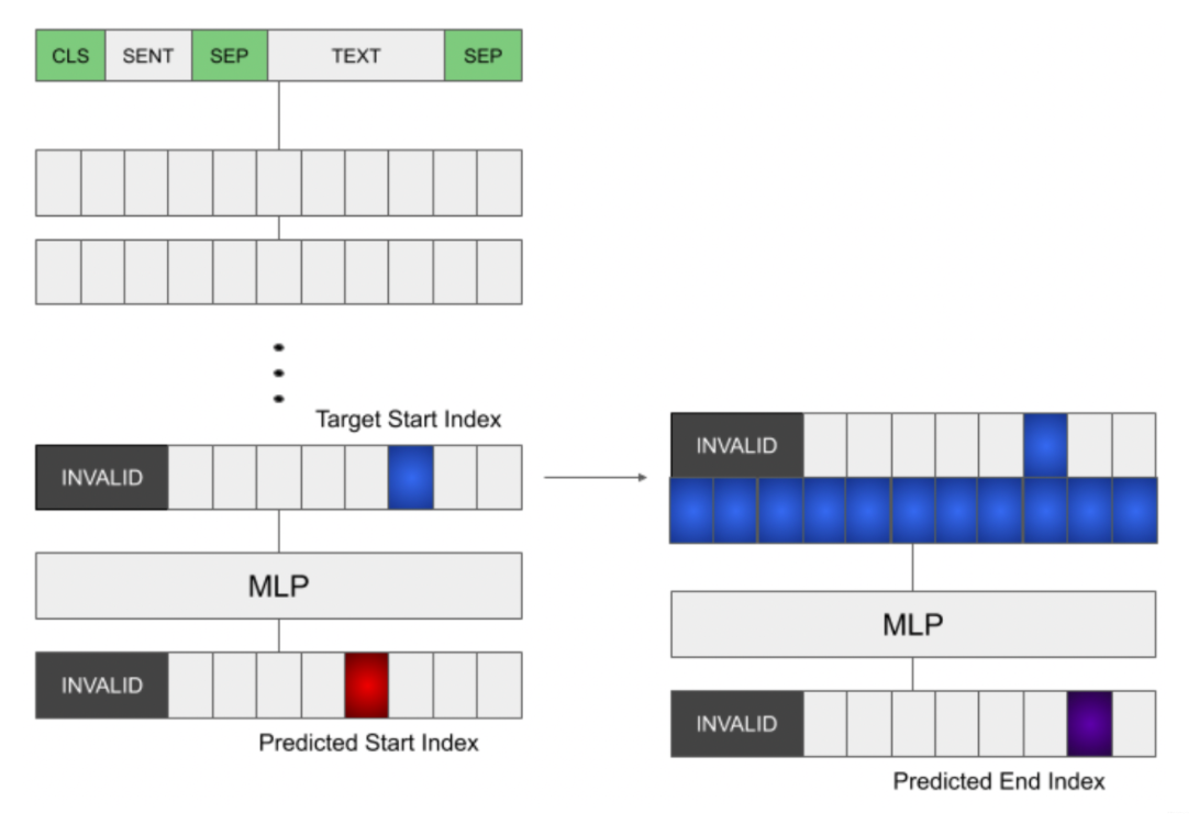
Inference:
- Predicting the start index normally.
- Take top-$k$ hidden states corresponding to top-$k$ start indices with highest probabilities.
- Each hidden state is then concatenated into the representations at every position.
- The new representation is fed to a MLP, similar to training. Then select top-$k$ end indices for each selected hidden state, resulting in $k \times k$ top start-end pairs.
- The best k is $3$, which resulted in a $3 \times 3$ start-end pairs. They ranked them by taking the product of the two probs.

Idea 2: Character level model with GRU head
Address the noisy targets by adding a prediction head that enables character wise span-prediction and completely learns the noise. They trained all models using a 5-seed average. Their best submission consists of a total of 3x5x2 models (backbones x seeds x team mates).
General explanation for idea 2
They realized that the key to a decent performance is the capability to predict a character-wise span. A good example, which they are also using in the illustration below is the tweet text “is back home now gonna miss everyone” which weirdly had the label “onna”. They knew that if a model would be able to predict “onna”, that would put them in a top spot.
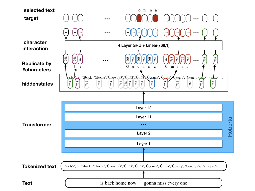
In fact a character-wise prediction would solves two issues:
- Definition of label: you now can just put the selected text as it as label.
- Predicting noise: you now are able to predict “half words” which was the key of the competition.
The key idea of this method is that “The model uses a standard transformer backbone which takes the word-level tokenized text and outputs hidden states with a certain dimension (in case of roberta-base 768). Instead of predicting the start and end word now, as done by “standard” models I replicate the hiddenstate of each word as often as the word has characters, so we get a hidden state for each character. In order to differentiate between characters I add a few 768 -> 768 RNN layers. Finally, two linear layers predict the start and end character of the selected text.”
In the following, I illustrate how the idea “replicate the hiddenstate of each word as often as the word has characters, so we get a hidden state for each character” is implemented. (Suppose we have $2$ words both having length $4$, with unique hidden states.)
>>> x = torch.tensor([[[1,2,5,7], [5,6,7,9]]])
>>> x
tensor([[[1, 2, 5, 7],
         [5, 6, 7, 9]]])

>>> x.size()
torch.Size([1, 2, 4])

>>> x.unsqueeze(-1)
tensor([[[[1],
          [2],
          [5],
          [7]],

         [[5],
          [6],
          [7],
          [9]]]])

>>> x.unsqueeze(-1).size()
torch.Size([1, 2, 4, 1])

>>> x.unsqueeze(-1).expand(-1,-1,-1, 5)
tensor([[[[1, 1, 1, 1, 1],
          [2, 2, 2, 2, 2],
          [5, 5, 5, 5, 5],
          [7, 7, 7, 7, 7]],

         [[5, 5, 5, 5, 5],
          [6, 6, 6, 6, 6],
          [7, 7, 7, 7, 7],
          [9, 9, 9, 9, 9]]]])
For the following ideas, we assume that we are writing a customized roberta model and here is the beginning of the customized roberta class:
Idea 3: fastai style freeze-unfreeze scheme
class CustomRoberta(nn.Module):

    def __init__(self, path='path/to/roberta-base/pytorch_model.bin'):
        super(CustomRoberta, self).__init__()

        config = RobertaConfig.from_pretrained(
            'path/to/roberta-base/config.json', output_hidden_states=True)

        self.roberta = RobertaModel.from_pretrained(path, config=config)
        self.weights_init_custom()

    # ignore the detail
    def forward(*args):
        pass
fastai style freeze-unfreeze scheme is the following:
def freeze(self):
    for child in self.roberta.children():
        for param in child.parameters():
            param.requires_grad = False

def unfreeze(self):
    for child in self.roberta.children():
        for param in child.parameters():
            param.requires_grad = True
idea 4: Customized Layer Initialization
The following code is an initialization of the last three layers of the model.
def weights_init_custom(self):
    init_layers = [9, 10, 11]
    dense_names = ["query", "key", "value", "dense"]
    layernorm_names = ["LayerNorm"]
    for name, module in self.roberta.named_parameters():
        if any(f".{i}." in name for i in init_layers):
            if any(n in name for n in dense_names):
                if "bias" in name:
                    module.data.zero_()
                elif "weight" in name:
                    module.data.normal_(mean=0.0, std=0.02)
            elif any(n in name for n in layernorm_names):
                if "bias" in name:
                        module.data.zero_()
                elif "weight" in name:
                    module.data.fill_(1.0)
Let’s break it into parts. Let’s see an example of a pair of name and module in self.roberta.named_parameters():
>>> name, module
('embeddings.word_embeddings.weight', Parameter containing:
 tensor([[ 0.1476, -0.0365,  0.0753,  ..., -0.0023,  0.0172, -0.0016],
         [ 0.0156,  0.0076, -0.0118,  ..., -0.0022,  0.0081, -0.0156],
         [-0.0347, -0.0873, -0.0180,  ...,  0.1174, -0.0098, -0.0355],
         ...,
         [ 0.0304,  0.0504, -0.0307,  ...,  0.0377,  0.0096,  0.0084],
         [ 0.0623, -0.0596,  0.0307,  ..., -0.0920,  0.1080, -0.0183],
         [ 0.1259, -0.0145,  0.0332,  ...,  0.0121,  0.0342,  0.0168]],
        requires_grad=True))
The followings are some examples of weights in the last three layers that they want to initialize:
encoder.layer.9.attention.self.query.weight
encoder.layer.9.attention.self.query.bias
encoder.layer.9.attention.self.key.weight
encoder.layer.9.attention.self.key.bias
encoder.layer.9.attention.self.value.weight
encoder.layer.9.attention.self.value.bias
encoder.layer.9.attention.output.dense.weight
encoder.layer.9.attention.output.dense.bias
encoder.layer.9.attention.output.LayerNorm.weight
encoder.layer.9.attention.output.LayerNorm.bias
Noteworthy ideas in 4th place solution
They also use the idea of re-ranking like in 2nd place team, but their re-ranking method is quite different, so I would like to do a summary of their ideas also.
They add four heads to each of their transformer model and here is the detail:
Head 1:
Take hidden states from the last two layers. Add a linear layer without any dropout for predicting start and end tokens (with label smoothing). This is common and used by each team.
Head 2:
Take hidden states from the last layer. Add a linear layer to predict binary target for each token: if it should be in selected text or not. Takes hidden states from the last layer. The loss in binary cross-entropy.
Head 3:
Take hidden states from the last layer. Add a linear layer to predict a sentiment of each token. Predicts three classes – neutral, positive and negative. Tokens from selected text are labeled as having the same sentiment as the tweet, while all other tokens are assigned neutral class. The loss in binary cross-entropy for each token separately.
Head 4:
Take hidden states from the last two layers. Concatenates mean and max pooling over all tokens in a tweet skipping cls and sentiment tokens. Add two linear layers with ReLU in between to predict the sentiment of the whole tweet (with MSD).
Training phase
During training, the total loss is calculated as the weighted sum of losses from all four heads. Training is performed on $8$ folds with AdamW optimizer and using (Stochastic Weight Averaging) SWA over a get_cosine_with_hard_restarts_schedule_with_warmup scheduler for 10 epochs.

Inference phase
Score 1 (from Head 1):
The first head is used to create a set of (start, end) candidates. Softmax is applied across all pairs to obtain probabilities for candidates and top $3$ of them are selected to be used for the further processing. Call the probability of a candidate from this head qa_prob.
Score 2 (from Head 2):
The output of the second head is the set of logits: one for each token. To obtain a score for each of the selected (start, end) candidates they took the sigmoid from the tokens and calculated the average log of the resultant token probabilities across candidate tokens. Call the output number as score_per_token.
Score 3 (from Head 3):
The output of the third head is used in a very similar way to the previous. The only difference is to take the softmax over each token logits instead of sigmoid since there are three classes of sentiments. Then the probability corresponding to the sentiment of the tweet is selected. Then the same averaging operation as for previous head is applied to obtain a score for candidates. Call it sentiment_per_token.
From the above, at inference time they now have three (start, end) candidates with three scores assigned to each of them.
Second level model
Similar to $2$nd team’s solution, they build a second level model on top of previous models.
Architecture
Used ELECTRA with the following input:
[CLS] ([POSITIVE]|[NEUTRAL]|[NEGATIVE]) tweet [SEP] selected_text_candidate [SEP]
Single head (linear->tanh->dropout->linear) on top of the transformer is fed with the concatenation of the cls token and the hidden states from the last two layers to predict if the current candidate for selected text is correct or not. Loss is computed with cross-entropy.
Training phase
Dataset for training is built with all tweets each having three candidates from the previous model and also tweet with true selected_text is added if it is not present among candidates. Trained it for 3 epochs with AdamW and SWA.
Inference phase
Three candidates for each tweet are scored with this model. It outputs two logits which are softmaxed and then the log of class 1 proba is taken as the score for the candidate. Will call it external_score in the following.
So after this step they have three candidates and each of them has four scores.
The final score for each candidate is the weighted sum of qa_prob, score_per_token, sentiment_per_token and external_score inside the model type (BERT, RoBERTa or ELECTRA) and then the weighted sum of these sums. The final prediction is the candidate with the largest score, which then goes through post-processing.
Reference:
- 1st place solution: https://www.kaggle.com/c/tweet-sentiment-extraction/discussion/159254
- 1st place solution code: https://www.kaggle.com/theoviel/character-level-model-magic
- 2nd place solution: https://www.kaggle.com/c/tweet-sentiment-extraction/discussion/159310
- 2nd place solution code: https://www.kaggle.com/hiromoon166/inference-8models-seed100101-bucketing-2-ver2/input?select=pre_processed.txt#Inference-of-Reranking-model
- 2nd place post-processing: https://www.kaggle.com/futureboykid/2nd-place-post-processing
- 3rd place solution: https://www.kaggle.com/c/tweet-sentiment-extraction/discussion/159910
- 3rd place solution code: https://github.com/suicao/tweet-extraction
- 4th place solution: https://www.kaggle.com/c/tweet-sentiment-extraction/discussion/159499
- 5th place solution: https://www.kaggle.com/c/tweet-sentiment-extraction/discussion/159268
- Label Smoothing code: https://www.kaggle.com/shonenkov/tpu-training-super-fast-xlmroberta, https://github.com/pytorch/pytorch/issues/7455
- Label Smoothing: https://www.flixstock.com/label-smoothing-an-ingredient-of-higher-model-accuracy, https://www.kaggle.com/shahules/tackle-with-label-smoothing-proved
- Multi-Sample Dropout for Accelerated Training and Better Generalization: https://arxiv.org/pdf/1905.09788.pdf
- https://stackoverflow.com/questions/50747947/embedding-in-pytorch
- sequence-bucketing: https://www.kaggle.com/bminixhofer/speed-up-your-rnn-with-sequence-bucketing#Implementation-&-comparing-static-padding-with-sequence-bucketing
- Re-ranking in QA paper: https://arxiv.org/pdf/1906.03008.pdf
- Common model structure: https://www.kaggle.com/c/tweet-sentiment-extraction/discussion/143281
- SWA: https://pytorch.org/blog/stochastic-weight-averaging-in-pytorch/