Consider an optimization problem in the standard form (we call this a primal problem):
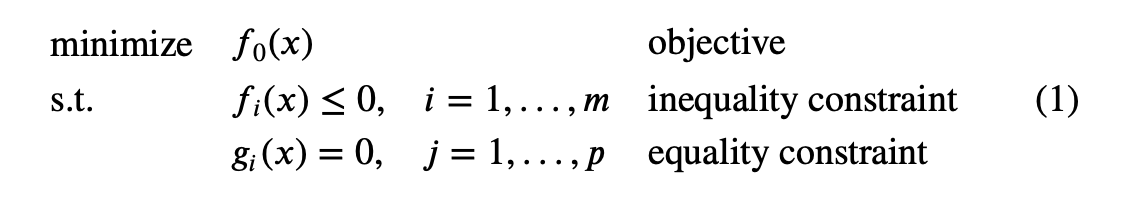
We denote the optimal value of this as $p^\star$. We don’t assume the problem is convex.
The Lagrange dual function
We define the Lagrangian $L$ associated with the problem as $$ L(x,\lambda, v) = f_0(x) + \sum^m_{i=1}\lambda_if_i(x) + \sum^p_{i=1}v_ih_i(x)$$ We call vectors $\lambda$ and $v$ the dual variables or Lagrange multiplier vectors associated with the problem (1).
We define the Lagrange dual function (or just dual function) $g$ as the minimum value of the Lagrangian over $x$: for $\lambda \in \mathbf{R}^m, v\in\mathbf{R}^p$, $$g(\lambda,v) = \mathop{\rm inf}\limits_{x\in \mathcal{D}} L(x, \lambda, v) = \mathop{\rm inf}\limits_{x\in \mathcal{D}} \left( f_0(x) + \sum^m_{i=1}\lambda_if_i(x) + \sum^p_{i=1}v_ih_i(x)\right)$$
Note that once we choose an $x$, $f_i(x)$ and $h_i(x)$ are fixed and therefore the dual function is a family of affine functions of ($\lambda$, $v$), which is concave even the problem (1) is not convex.
Lower bound property
The dual function yields lower bounds on the optimal value $p^\star$ of the problem (1): For any $\lambda \succeq 0$ and any $v$ we have $$ g(\lambda,v) \leq p^\star$$
Suppose $\tilde{x}$ is a feasible point for the problem (1), i.e., $f_i(\tilde{x}) \leq 0$ and $h_i(\tilde{x}) = 0$, and $\lambda \succeq 0$. Then we have
$$ L(\tilde{x}, \lambda, v) = f_0(\tilde{x}) + \sum^m_{i=1}\lambda_if_i(\tilde{x}) + \sum^p_{i=1}v_ih_i(\tilde{x}) \leq f_0(\tilde{x})$$
Hence $$ g(\lambda,v) = \mathop{\rm inf}\limits_{x\in \mathcal{D}} L(x, \lambda, v) \leq L(\tilde{x}, \lambda, v) \leq f_0(\tilde{x})$$
Since $g(\lambda,v) \leq f_0(\tilde{x})$ holds for every feasible point $\tilde{x}$, the inequality $g(\lambda,v) \leq p$ follows. The inequality holds, but is vacuous, when $g(\lambda,v) = -\infty$. The dual function gives a nontrivial lower bound on $p^\star$ only when $\lambda \succeq 0$ and $(\lambda,v) \in \textbf{dom},g$, i.e., $g(\lambda,v) > - \infty$. We refer to a pair $(\lambda,v)$ with $\lambda \succeq 0$ and $(\lambda,v) \in \textbf{dom},g$ as dual feasible.
Derive an analytical expression for the Lagrange dual function
Practice problem 1: Least-squares solution of linear equations
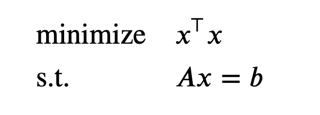
The Lagrangian is $L(x,v) = x^\top x + v^\top(Ax-b)$. The dual function is given by $g(v) = \text{inf}_x L(x,v)$. Since $L(x,v)$ is a convex quadratic function of $x$, we can find the minimizing $x$ from the optimality condition
$$ \nabla_x L(x,v) = 2x + A^\top v = 0$$
which yields $x = -(1/2)A^\top v$. Therefore the dual function is
$$ g(v) = L(-(1/2)A^\top v, v) = -(1/4)v^\top AA^\top v - b^\top v$$
Therefore, $p^\star \geq -(1/4)v^\top AA^\top v - b^\top v$. The next step is to maximize $-(1/4)v^\top AA^\top v - b^\top v$.
Practice problem 2: Standard form Linear Programming
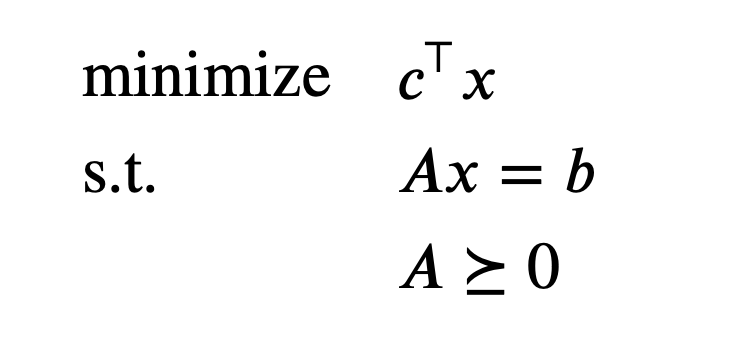
The Lagrangian is $$ L(x, \lambda, v) = c^\top x - \sum^n_{i=1}\lambda_ix_i + v^\top(Ax-b) = -b^\top v + (c + A^\top v - \lambda)^\top x$$
The dual function is $$ g(\lambda, v) = \mathop{\rm inf}\limits_{x} L(x, \lambda, v) = -b^\top v + \mathop{\rm inf}\limits_{x}, (c + A^\top v - \lambda)^\top x$$
We see that $g(\lambda,v)$ is a linear function. Since a linear function is bounded below only when it is zero. Thus, $g(\lambda,v) = -\infty$ except when $c + A^\top v - \lambda = 0$. Therefore,
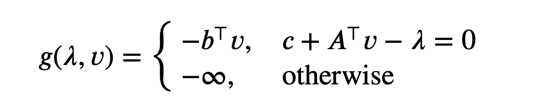
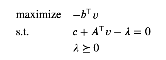
The lower bound property is nontrivial only when $\lambda$ and $v$ satisfy $\lambda \succeq 0$ and $c + A^\top v - \lambda$. When this occurs, $-b^\top v$ is a lower bound on the optimal value of the LP. We can form an equivalent dual problem by making these equality constraints explicit:
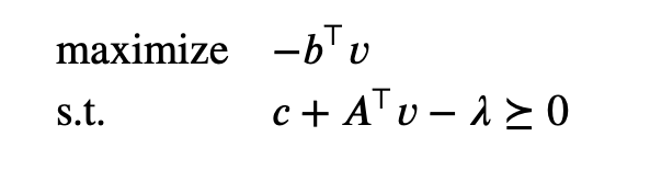
This problem, in turn, can be expressed as
The Lagrange dual problem
For each pair $(\lambda,v)$ with $\lambda \succeq 0$, the Lagrange dual function gives us a lower bound on the optimal value $p^\star$ of the optimization problem (1). Thus we have a lower bound that depends on some parameters $\lambda, v$.
This leads to the optimization problem
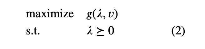
This problem is called the Lagrange dual problem associated with the problem (1). In this context the original problem (1) is sometimes called the primal problem. We refer to $(\lambda^\star, v^\star)$ as dual optimal or optimal Lagrange multipliers if they are optimal for the problem (2). The Lagrange dual problem (2) is a convex optimization problem, since the objective to be maximized is concave and the constraint is convex. This is the case whether or not the primal problem (5.1) is convex.
Note: the dual problem is always convex.
Weak/ Strong duality
The optimal value of the Lagrange dual problem, which we denote $d^\star$, is, by definition, the best lower bound on $p^\star$ that can be obtained from the Lagrange dual function. The inequality
$$ d^\star \leq p^\star$$
which holds even if the original problem is not convex. This property is called weak duality.
We refer to the difference $p^\star - d^\star$ as the optimal duality gap of the original problem. Note that th optimal duality gap is always nonnegative.
We say that strong duality holds if
$$ d^\star = p^\star$$
Note that strong duality does not hold in general. But if the primal problem (11) is convex with $f_1, …, f_k$ convex, we usually (but not always) have strong duality.
Slater’s condition
Slater’s condition: There exists an $x \in \mathbf{relint}, D$ such that $$f_i(x) < 0, \quad i = 1,…,m, \quad Ax = b $$
Such a point is called strictly feasible.
Slater’s theorem: If Slater’s condition holds for a convex problem, then the strong duality holds.
Complementary slackness
Suppose the strong duality holds. Let $x^\star$ be a primal optimal and $(\lambda^\star, v^\star)$ be a dual optimal point. This means that

We conclude that the two inequalities in this chain hold with equality. Since the inequality in the third line is an equality, we conclude that $x^\star$ minimizes $L(x, \lambda^\star, v^\star)$ over $x$.
Another important conclusion is
$$ \lambda_i^\star f_i(x^\star) = 0, \quad i = 1,…,m$$
KKT optimality conditions
We now assume that the functions $f_0, …, f_m, h_1, …,h_p$ are differentiable, but we make no assumptions yet about convexity.
KKT conditions for nonconvex problems
Suppose the strong duality holds. Let $x^\star$ be a primal optimal and $(\lambda^\star, v^\star)$ be a dual optimal point. Since $x^\star$ minimizes $L(x, \lambda^\star, v^\star)$ over $x$, it follows that its gradient must vanish at $x^\star$, i.e.,
$$ \nabla f_0(x^\star) + \sum^m_{i=1}\lambda_i^\star \nabla f_i(x^\star) + \sum^p_{i=1}v_i^\star \nabla h_i(x^\star) = 0$$
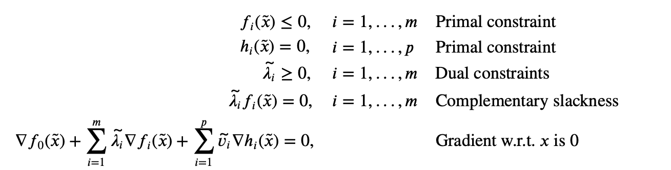
The KKT conditions are the following:

For any optimization problem with differentiable objective and constraint functions for which strong duality obtains, any pair of primal and dual optimal points must satisfy the KKT conditions.
KKT conditions for convex problems
When the primal problem is convex, the KKT conditions are also sufficient for the points to be primal and dual optimal. That is, if $f_i$ are convex and $h_i$ are affine, and $\tilde{x}, \tilde{\lambda}, \tilde{v}$ are any points that satisfy the KKT conditions
then $\tilde{x}$ and $(\tilde{\lambda_i}, \tilde{v_i})$ are primal and dual optimal, with zero duality gap. To see this, note that the first two conditions state that $\tilde{x}$ is primal feasible. Since $\tilde{\lambda_i}$ ≥ 0, $L(x,\tilde{\lambda},\tilde{v})$ is convex in $x$; the last KKT condition states that its gradient with respect to $x$ vanishes at $x = \tilde{x}$, so it follows that $\tilde{x}$ minimizes $L(x,\tilde{\lambda},\tilde{v})$ over $x$. From this we conclude that

This shows that $\tilde{x}$ and $(\tilde{\lambda},\tilde{v})$ have zero duality gap, and therefore are primal and dual optimal.
We conclude the following:
- For any convex optimization problem with differentiable objective and constraint functions, any points that satisfy the KKT conditions are primal and dual optimal, and have zero duality gap.
- If a convex optimization problem with differentiable objective and constraint functions satisfies Slater’s condition, then the KKT conditions provide necessary and sufficient conditions for optimality: Slater’s condition implies that the optimal duality gap is zero and the dual optimum is attained, so $x$ is optimal iff there are $(\lambda, v)$ that, together with $x$, satisfy the KKT conditions.
Solving the primal problem via the dual
Note that if strong duality holds and a dual optimal solution $(\lambda^\star, v^\star)$ exists, then any primal optimal point is also a minimizer of $L(x, \lambda^\star, v^\star)$. This fact sometimes allows us to compute a primal optimal solution from a dual optimal solution.
More precisely, suppose we have strong duality and an optimal $(\lambda^\star, v^\star)$ is known. Suppose that the minimizer of $L(x, \lambda^\star, v^\star)$, i.e., the solution of
is unique (For a convex problem this occurs). Then if the solution is primal feasible, it must be primal optimal; if it is not primal feasible, then no primal optimal point can exist, i.e., we can conclude that the primal optimum is not attained.
Reference:
- Convex Optimization* by Stephen Boyd and Lieven Vandenberghe.